2. Solutions#
Solutions are now complete. See Blackboard for information about non-examinable topics and instructions for the exam.
2.1. Preliminary problems#
P1. The correct statements are (ii) and (v).
In statement (iv), the quantifiers \(\forall\) and \(\exists\) are the wrong way round, while in (i) they are missing altogether. Statement (iii) asserts that last part, \(|x_n-l|<\varepsilon\) \(\forall n\geq N\), should hold for all \(\varepsilon\) and for all \(N\) — so again, there is an issue with the quantifiers.
Bonus exercise: prove that (iv) holds if and only if \((x_n)\) is the constant sequence \(x_n=l\) for all \(n\in\mathbb{N}\).
P2. (Homework 1 question).
Let \(\varepsilon>0\). According to the definition, we must prove there is an \(N\in\mathbb{N}\) for which \(\left|\frac{2n}{3n-1}-\frac{2}{3}\right|<\varepsilon\) whenever \(n\geq N\).
Now,
This will be strictly less than \(\varepsilon\) whenever \(3n-1>\frac{2}{3\varepsilon}\)., or in other words, whenever
Let \(N\) be any integer greater than \(\frac{2+3\varepsilon}{9\varepsilon}\). Then \(\left|x_n-\frac{2}{3}\right|<\varepsilon\) for all \(n\geq N\), and we have proven that \(x_n\rightarrow\frac{2}{3}\) as \(n\rightarrow\infty\) using the definition.
P3. (Homework 1 question).
The Bolzano–Weierstrass theorem states that every bounded sequence has a convergent subsequence. Its proof combines the following two results:
The monotone convergence theorem (Theorem 3.10 in the MAS107 notes), which states that bounded monotone sequences must converge.
More specifically, every monotone increasing sequence that is bounded above converges to its supremum, and every monotone decreasing sequence bounded below converges to its infimum.Theorem 3.13 from MAS107: Every sequence has a monotone subsequence.
Proof of Bolzano–Weierstrass:
If \((x_n)\) is a bounded sequence, then it has a monotone subsequence, \((x_{n_k})\), by Theorem 3.13. This subsequence must also be bounded since \((x_n)\) is bounded, and hence it converges by the monotone convergence theorem.
P4.(i) Let \(a, b \geq 0\). Then,
while,
Therefore
Since \(\sqrt{a}\), \(\sqrt{b}\) and \(\sqrt{a+b}\) are all non-negative and the square root function is increasing, we can square root both sides to get
(ii) Note that the inequality we have been asked to prove is symmetric in \(a\) and \(b\), in the sense that exchanging the roles of \(a\) and \(b\) does not affect the value of either side.
This means we can assume without loss of generality that \(\sqrt{|a|}\geq\sqrt{|b|}\). Then,
and we need only show that
We use a trick similar to the proof of Corollary 1.1, and write
By the triangle inequality, we have that \(|a| = \big|(a-b) + b\big| \leq |a-b|+|b|\).
Since the square root function is increasing, we can square root both sides to get
Applying the result from (i) to the right-hand side, it follows that
Equation (2.1) now follows by subtracting \(\sqrt{|b|}\) from both sides.
(iii) Let \((a_n)\) be a real sequence converging to \(l\in\mathbb{R}\). By (ii),
for all \(n\in\mathbb{N}\).
Let \(\varepsilon>0\). Since \(a_n\rightarrow l\), there is \(N\in\mathbb{N}\) such that \(|a_n-l|<\varepsilon^2\) whenever \(n\geq N\). Hence for \(n\geq N\),
Thus \(\displaystyle\lim_{n\rightarrow\infty}\sqrt{|a_n|} = \sqrt{|l|}\).
P5. When it exists, the supremum of a set \(A\subseteq\mathbb{R}\) is defined to be the unique number \(\alpha\in\mathbb{R}\) such that
\(\alpha\) is an upper bound for \(A\), and
if \(M\) is any other upper bound for \(A\), then \(\alpha\leq M\).
We write \(\sup A\) for the supremum of \(A\), when it exists.
The definition of the infimum is similar: when it exists, the infimum of \(A\) is the unique number \(\beta\in\mathbb{R}\) such that
(i) \(\beta\) is a lower bound for \(A\), and
(ii) if \(L\) is any other lower bound for \(A\), then \(\alpha\geq L\).
We write \(\inf A\) for the infimum of \(A\), when it exists.
The axiom of completeness for the real numbers says that every non-empty bounded above subset of \(\mathbb{R}\) has a supremum. Equivalently, it says that every non-empty bounded below subset of \(\mathbb{R}\) has an infimum.
For more details, see page 32 of your Semester 2 MAS107 notes.
P6.(i) \(\displaystyle\sup\left\{\frac{m}{n}:m,n\in\mathbb{N} \text{ s.t } m<n\right\}=1\), \(\displaystyle\inf\left\{\frac{m}{n}:m,n\in\mathbb{N} \text{ s.t } m<n\right\}=0\).
(ii) \(\displaystyle\sup\left\{\frac{(-1)^m}{n}:m,n\in\mathbb{N} \text{ s.t } m<n\right\}=\frac{1}{3}\), \(\displaystyle\inf\left\{\frac{(-1)^m}{n}:m,n\in\mathbb{N} \text{ s.t } m<n\right\}=-\frac{1}{2}\).
(iii) \(\displaystyle\sup\left\{\frac{n}{3n + 1} :n\in\mathbb{N}\right\}=\frac{1}{3}\), \(\displaystyle\inf\left\{\frac{n}{3n + 1} :n\in\mathbb{N}\right\}=\frac{1}{4}\).
P7.(i) This is false — for a counter-example, take any singleton set. Then \(\sup A=\inf A=1\).
A correct version of the statement would be \(\inf A \leq \sup A\).
(ii) True. The analogous statement for \(\sup\) was called the characteristic property of the supremum in your MAS107 lecture notes — see Lemma 2.8 on page 36.
(iii) True. Since \(\sup B\) is an upper bound for \(B\), and \(A\) is a subset of \(B\), \(\sup B\) must be an upper bound for \(A\). But \(\sup A\) is a the least upper bound for \(A\), hence \(\sup A\leq \sup B\). The analogous property for \(\inf\) is that \(\inf A\geq\inf B\) whenever \(A\subseteq B\).
(iv) False. For a counter-example, take \(B=\left\{\frac{1}{n}:n\in\mathbb{N}\right\}\), for which \(\inf B=0\).
(v) True. Let \(s=\max\{\sup A,\sup B\}\). Then \(s\geq \sup A\) and \(s\geq \sup B\), so \(s\) is an upper bound for both \(A\) and \(B\). Therefore, \(s\) is an upper bound for \(A\cup B\). But \(\sup(A\cup B)\) is the least upper bound of \(A\cup B\), and so \(s\geq\sup(A\cup B)\). Also, since \(A\) and \(B\) are both subsets of \(A\cup B\), we have by statement (iii) that \(s=\max\{\sup A,\sup B)\leq\sup(A\cup B)\). Hence \(\max\{\sup A,\sup B)=\sup(A\cup B)\).
2.2. Limits of functions#
1. One has to identify the real numbers where the given formula does not make sense, usually because of a zero in a denominator somewhere, and exclude them.
(i) \(A=\mathbb{R} \setminus \{0, -1\}\).
(ii) \(g_{2}(x) = \displaystyle\frac{(x-1)(x+4)}{(x-1)(x+2)(x+3)}\), so \(A=\mathbb{R} \setminus \{1, -2, -3\}\).
(iii) \(g_{3}(x) = \displaystyle\frac{x+4}{(x+2)(x+3)}\), so \(A=\mathbb{R} \setminus \{-2, -3\}\).
(iv) \(A=\mathbb{R} \setminus \{1\}\).
(v) \(A=\mathbb{R} \setminus \{0\}\).
2. (Homework 1 question).
Note
This question was ambiguous about whether or not proofs are required. Strictly speaking, “being able to prove rigorously which real numbers are the limit points of a given set” is not a key learning outcome for this module, so the proofs included below are largely for interest. What is important is that you know the definition of a limit point, and understand it well enough that you can identify which real numbers are limit points of a given set, and which are not.
(i) \(X=(0,1)\cup[2,3)\cup\{4,5\}\). Set of limit points: \(L=[0,1]\cup[2,3]\).
Proof (dropdown)
Let \(L\) be the set of all limit points of \(X\). We prove that \(L=[0,1]\cup[2,3]\) by proving \(L\subseteq[0,1]\cup[2,3]\) and \(L\supseteq[0,1]\cup[2,3]\).
\((\supseteq)\) Let \(a\in[0,1]\cup[2,3]\). We prove \(a\) is a limit point of \(X=(0,1)\cup[2,3)\cup\{4,5\}\) by explicitly writing down a sequence \((x_n)\) in \(X\setminus\{a\}\) with limit \(a\). In fact, \(x_n=a+\frac{1}{n+3}\) works for any choice \(a\in[0,1)\cup[2,3)\). If \(a=0\) or \(a=3\), then use \(x_n=a-\frac{1}{n}\) instead. Either way, we have shown that \(a\in L\).
\((\subseteq)\) If \(a\in L\), then there is a sequence \((x_n)\) in \(X\setminus\{a\}\), with \(a=\lim_{n\rightarrow\infty}x_n\). Since \(x_n\in X\) for all \(n\in\mathbb{N}\), we must have \(0<x_n\leq 5\) for all \(n\in\mathbb{N}\), and so \(0\leq a\leq 5\).
If \(a\in(1,2)\), then the definition of convergence says that for any \(\varepsilon>0\), we can find \(N\in\mathbb{N}\) such that \(x_n\in(a-\varepsilon,a+\varepsilon)\) for all \(n\geq N\). We know this holds for any \(\varepsilon>0\), so in particular we can choose \(\varepsilon>0\) such that \((a-\varepsilon,a+\varepsilon)\subseteq(1,2)\). For this choice of \(\varepsilon\) and resulting \(N\), we have that \(x_n\in(1,2)\) for all \(n\geq N\). But this contradicts \((x_n)\) being a sequence in \(X\). So \(a\notin (1,2)\).
Finally, suppose \(a>3\). By a similar argument, we can choose \(\varepsilon>0\) small enough so that \((a-\varepsilon,a+\varepsilon)\subseteq(3,\infty)\). Since \(x_n\rightarrow a\), we know there exists \(N\in\mathbb{N}\) such that \(|x_n-a|<\varepsilon\) for all \(n\geq N\). Therefore, for all \(n\geq N\), we have \(x_n\in(a-\varepsilon,a+\varepsilon)\subseteq (3,\infty)\). In other words, \(x_n>3\) for all \(n\geq N\). The only elements of \(X\) that are strictly larger than \(3\) are \(4\) and \(5\). This means that \(x_n\in\{4,5\}\) for all \(n\geq N\). But then, since \((x_n)\) converges to \(a\), it must be eventually constant and equal to \(a\), contradicting \(x_n\neq a\) for all \(n\in\mathbb{N}\). So \(a\leq 3\).
It follows that \(a\in[0,1]\cup[2,3]\).\(\square\)
(ii) \(X=\mathbb{Z}\). Set of limit points: \(L=\emptyset\).
Proof (dropdown)
If \(a\) is a limit point of \(\mathbb{Z}\), then there is a sequence \((x_n)\) in \(\mathbb{Z}\), with \(x_n\neq a\) for all \(n\in\mathbb{N}\), and \(\lim_{n\rightarrow\infty}x_n=a\). But all convergent sequences in \(\mathbb{Z}\) are eventually constant, so this is impossible. \(\square\)
(iii)\(X=\mathbb{R}\setminus\mathbb{Z}\). Set of limit points: \(L=\mathbb{R}\).
Proof (dropdown)
If \(a\in\mathbb{Z}\), then \(x_n:=a+\frac{1}{2n}\) defines a sequence in \(X\) with limit \(a\), and clearly \(x_n\neq a\) for all \(n\in\mathbb{N}\). This shows \(\mathbb{Z}\subseteq L\). If \(a\in\mathbb{R}\setminus\mathbb{Z}\), then \(a\) must lie in some open interval \((k,k+1)\), where \(k\in\mathbb{Z}\) (in fact \(k=\lfloor x\rfloor\)).
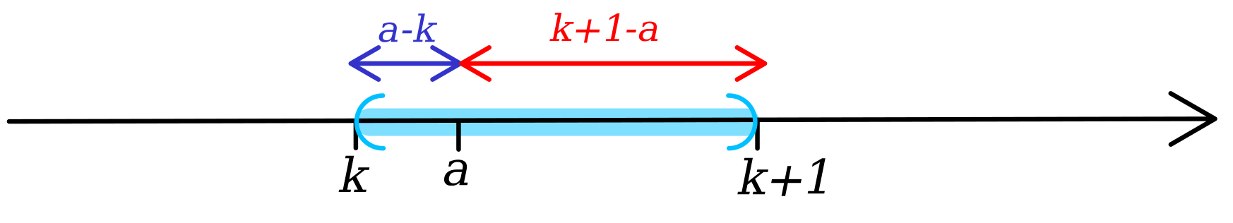
Fig. 2.1 Sketch to decide/justify choice \(\delta:=\min\{x-a,k+1-a\}\) (Problem 2(iii))#
Let \(\delta=\min\{x-a,k+1-a\}\) (this choice is strongly motivated by a sketch — see Fig. 2.1.). Then \(x_n:=a+\frac{\delta}{n}\) defines a sequence in \((k,k+1)\), with limit \(a\), and such that \(x_n\neq a\) for all \(n\in\mathbb{N}\).\(\square\)
(iv) \(X=\{x\in\mathbb{Q}:0<x<1\}\). Set of limit points: \(L=[0,1]\)
Proof (dropdown)
If \((x_n)\) is a convergent sequence in \(X\), then \(0<x_n<1\) for all \(n\in\mathbb{N}\), and so \(0\leq\lim_{n\rightarrow\infty}x_n\leq 1\). This shows that \(L\subseteq [0,1]\). On the other hand, if \(a\in[0,1]\), then by density of the rationals, for all \(n\in\mathbb{N}\) there is a rational number \(x_n\) satisfying \(a<x_n<a+\frac{1}{n}\). Then, \(x_n\neq a\) for all \(n\in\mathbb{N}\), and by the squeeze theorem, \(x_n\rightarrow a\) as \(n\rightarrow\infty\). Also, since \(a\in[0,1]\), with the exception of the case \(a=1\) (treated separately below), we will eventually have \(0<x_n<1\) for all \(n\in\mathbb{N}\) sufficiently large. In other words, removing a finite number of initial terms if necessary, we have found a sequence in \(X\setminus\{a\}\) with limit \(a\).
For the case \(a=1\), use the same argument, but with sequence \((x_n)\) of rational numbers chosen so that \(1-\frac{1}{n}<x_n<1\), for each \(n\in\mathbb{N}\).\(\square\)
(v) \(X=\displaystyle\left\{\frac{1}{n}:n\in\mathbb{N}\right\}\). \(L=\{0\}\)
Proof (dropdown)
That \(0\in L\) follows by taking the sequence \(x_n=\frac{1}{n}\). On the other hand, if \(a\in L\), then there is a sequence \((x_n)\) in \(X\setminus\{a\}\) with limit \(a\). All elements of \(X\) are strictly positive, so \(x_n>0\) for all \(n\in\mathbb{N}\), and hence \(a\geq 0\). Suppose that \(a>0\). Then by definition of convergence, there is \(N\in\mathbb{N}\) such that \(|x_n-a|<\frac{a}{2}\) for all \(n\geq N\). But then \(x_n\in\left(\frac{a}{2},\frac{3a}{2}\right)\) for all \(n\geq N\). There are only finitely many elements of \(X\) that lie in this interval, and we know \((x_n)\) converges to \(a\). So, the only option is that \((x_n)\) is eventually constant and equal to \(a\). This is a contradiction, since \((x_n)\) is a sequence in \(X\setminus\{a\}\). It follows that \(a=0\).\(\square\)
3. (Homework 1 question).
(i) We are given \(f:\mathbb{R}\to\mathbb{R}\); \(f(x)=4x+7\). Intuition tells us that
To prove this, let \(\varepsilon>0\). We seek \(\delta>0\) such that \(0<|x-2|<\delta\) implies \(|f(x)-15|<\varepsilon\).
Note that
Therefore, putting \(\delta=\frac{\varepsilon}{4}\), we get that whenever \(0<|x-2|<\delta\),
For the limit as \(x\rightarrow 0\), we claim that \(\lim_{x\rightarrow 0}f(x)=7\). To prove this, note that \(|f(x)-7|=4|x|\). This means that given \(\varepsilon>0\), if \(0<|x|<\frac{\varepsilon}{4}\) then
It follows that \(\lim_{x\rightarrow 0}f(x)\) exists and is equal to \(7\).
(ii) We have \(f:\{0\}\cup[1,3]\to\mathbb{R}\); \(f(x)=3x^2-1\), so using intuition only, \(\lim_{x\rightarrow 2} f(x)=3\cdot 4-1=11\).
Let \(\varepsilon>0\). We seek \(\delta>0\) such that for all \(x\in\{0\}\cup[1,3]\),
Now, for \(x\in\{0\}\cup[1,3]\),
(Here, we have used the fact that \(|x+2| = x+2 \leq 5\), for \(x\in\{0\}\cup[1,3]\).)
Hence we can let \(\delta:=\frac{\varepsilon}{15}\) and conclude that if \(x\in\{0\}\cup[1,3]\) and \(0<|x-2|<\frac{1}{15}\), then
For this \(f\), \(\lim_{x\rightarrow 0}f(x)\) is not defined, since \(0\) is not a limit point of the domain of \(f\).
(iii) Finally, let \(f:(0,\infty)\to\mathbb{R}\); \(f(x)=x+\frac{1}{x}\). The limit of \(f(x)\) as \(x\rightarrow 2\) ought to be \(2+\frac{1}{2}=\frac{5}{2}\).
Let \(\varepsilon>0\), and consider
Observe that if \(x\in(0,\infty)\) and \(|x-2|<1\), then \(0<1-\frac{1}{2x}<1\), and so
To make sure the above inequality holds and is bounded above by \(\varepsilon\), let \(\delta:=\min\{\varepsilon,1\}\).
Suppose that \(x\in(0,\infty)\) with \(0<|x-2|<\delta\). Then by our choice of \(\delta\), \(0<|x-2|<1\) and \(0<|x-2|<\varepsilon\) both hold simultaneously. It follows that
and hence \(\lim_{x\rightarrow 2}f(x)=\frac{5}{2}\) is proved.
For the last part, note that \(f(x)=x+\frac{1}{x}\) does not converge to a finite limit as \(x\rightarrow 0\). In fact, \(\lim_{x\rightarrow 0}f(x)=\infty\). One way to prove this is to show that \(f(x)\) surpasses any possible bound as \(x\rightarrow 0\). Note that
Therefore, given an arbitrary number \(K>0\), we can take \(0<x<\frac{1}{K}\) to ensure that
This proves that \(\lim_{x\rightarrow 0} f(x) = \infty\), for this choice of \(f\).
4. We had \(A= \mathbb{R} \setminus \{1, -2, -3\}\), and \(f_2:A\to\mathbb{R}\); \(\displaystyle g_{2}(x)= \frac{(x + 4)}{(x + 2)(x + 3)}\).
It is considerably easier to use the sequential criterion for functional limits (Theorem 2.1) than it is to proceed directly using the Definition 2.1. We include both methods, for completeness.
Method 1: Sequences:
Let \((x_n)\) be a sequence in \(A\) converging to \(1\). Then, using algebra of limits for real sequences,
where the last equality is using algebra of limits. So \(\displaystyle\lim_{x \rightarrow 1}g_{2}(x) = \frac{5}{12}\).
Let \(x_n=-2 + \frac{1}{n}\), so that \((x_n)\) is a sequence in \(A\) converging to \(-2\). Then we see that \((f_2(x_n))\) diverges to \(+\infty\) and so \(\lim_{x \rightarrow -2}g_{2}(x)\) does not exist.
Similarly, considering \(x_n=-3 + \frac{1}{n}\), we see that \(\lim_{x \rightarrow -3}g_{2}(x)\) does not exist.
Method 2: \((\varepsilon-\delta)\) criterion:
Intuitively speaking, the limit as \(x\rightarrow 1\) “should” be \(\frac{(1 + 4)}{(1 + 2)(1 + 3)}=\frac{5}{12}\).
We prove \(\lim_{x\rightarrow 1}f_2(x) = \frac{5}{12}\).
Let \(\varepsilon>0\). We wish to find \(\delta>0\) so that if \(x\in A\) and \(0<|x-1|<\delta\), then \(\left|f_2(x)-\frac{5}{12}\right| <\varepsilon\).
Now,
We are going to constrain \(x\) to be very close to \(1\). In particular, we can assume \(0<x<2\), so
Finally, we choose \(\delta:= \frac{3}{14}\varepsilon\). Then, for \(0<|x-1|< \delta\),
5. The first part follows by using the sequential criterion for a limit of a function, and then applying the result of P4 (iii)..
To be precise let \((x_{n})\) be any sequence in \(\mathbb{R} \setminus \{a\}\) that converges to \(a\). Then since we are given that \(\lim_{x \rightarrow a} f(x) = l\), we must have that \(\lim_{n\rightarrow\infty} f(x_{n}) = l\). But then by P4 (iii)., we have \(\lim_{n\rightarrow\infty} \sqrt{f(x_{n}}) = \sqrt{l}\). So by definition of the limit of a function, \(\lim_{x \rightarrow a} \sqrt{f(x)} = \sqrt{l}\).
Using algebra of limits, \(\lim_{x \rightarrow 1}\displaystyle\frac{x+1}{x^{2}}=\frac{1+1}{1^2}=2\) and
then by the first part \(\lim_{x \rightarrow 1}\sqrt{\displaystyle\frac{x+1}{x^{2}}} = \sqrt{2}\).
6. Let \(f:A\to \mathbb{R}\) and suppose that \(\lim_{x \rightarrow a} f(x) = l\) and \(\lim_{x \rightarrow a} f(x) = l'\). Then given any sequence \((x_{n})\) in \(A \setminus \{a\}\) that converges to \(a\), we have \(\lim_{n\rightarrow\infty} f(x_{n}) = l\) and also \(\lim_{n\rightarrow\infty} f(x_{n}) = l'\). But then \(l = l'\), by uniqueness of limits.
7.
When \(x > 0, \displaystyle\frac{|x|}{x} = \displaystyle\frac{x}{|x|} = \displaystyle\frac{x}{x} = 1 = \text{sgn}(x)\), and when \(x < 0, \displaystyle\frac{|x|}{x} = \displaystyle\frac{x}{|x|} = -\displaystyle\frac{x}{x} = -1 = \text{sgn}(x)\). So \(\text{sgn}(x) = \displaystyle\frac{|x|}{x} = \displaystyle\frac{x}{|x|}\), when \(x\neq 0\).
Consider the sequences \(x_n=\frac{1}{n}\) and \(y_n=-\frac{1}{n}\). If \(\lim_{x\rightarrow 0}\text{sgn}(x)\) existed, then we would have
But in fact, \(\text{sgn}(x_n)=1\) and \(\text{sgn}(y_n)=-1\) for all \(n\in\mathbb{N}\), so
So \(\text{sgn}\) does not converge as \(x\rightarrow 0\).
For the left and right limits at \(0\):
The left limit is \(\displaystyle\lim_{x \rightarrow 0^-} \text{sgn}(x) = -1\), since for any sequence \((x_n)\) approaching \(0\) from the left, we have \(\text{sgn}(x_n) = -1\) for all \(n\).
The right limit is \(\displaystyle\lim_{x \rightarrow 0^+} \text{sgn}(x) = 1\), since for any sequence \((x_n)\) approaching \(0\) from the right, we have \(\text{sgn}(x_n) = 1\) for all \(n\).
8. (Homework 2 question).
(i) We are given \(f:\mathbb{R}\to\mathbb{R}\); \(f(x) = \begin{cases} 1 -x & \text{if }x < 1\\ x^{2}& \text{if }x \geq 1. \end{cases}\)
For \(a\neq 1\), the left and right limits exist and are both equal to \(f(a)\), using the algebra of limits. The only point at which left and right limits disagree is \(a = 1\), with
To prove the left limit, let \(\varepsilon>0\). For \(x<1\), \(f(x)=1-x\). Therefore, if \(-\varepsilon<x-1<0\), we have \(0<1-x<\varepsilon\), and hence \(|f(x)|=|1-x|<\varepsilon\).
For the right limit: We know that if \(x>1\), \(f(x)=x^2\). Given \(\varepsilon>0\), we seek \(\delta>0\) such that if \(0<x<\delta\), then \(|f(x)-1|<\varepsilon\). Now,
We can bound the \(|x+1|\) factor above by \(3\) provided we choose a \(\delta\) that is at most \(1\). Indeed: if \(0<x-1<1\), then \(2<x+1<3\), so \(|x+1|<3\).
We choose \(\delta=\min\left\{1,\frac{\varepsilon}{3}\right\}\). Then, for \(0<x-1<\delta\), we have \(0<x-1<1\) and \(0<|x-1|<\frac{\varepsilon}{3}\). So,
Note
We could have also used algebra of limits to prove/evaluate the left- and right-limits here. For example, to show \(\lim_{x\rightarrow 1^-}f(x)=1\), apply algebra of limits to the function \(x^2\) (domain \(\mathbb{R}\)). This tells us that \(\lim_{x\rightarrow 1}x^2=1\). Therefore, by Proposition 2.1, \(\lim_{x\rightarrow 1^-}x^2=1\). But then, since \(f(x)=x^2\) for all \(x<1\), we must have that \(\lim_{x\rightarrow 1^-}f(x)=\lim_{x\rightarrow 1^-}x^2=1\).
(ii) Consider \(g:\mathbb{R}\to\mathbb{R}\), \(g(x) = [x] = \left\{\begin{array}{cl} \lfloor x\rfloor & \text{ if } x\geq 0 \\ \lceil x \rceil & \text{ if } x<0 \end{array}\right.\).
A quick think about how \([x]\) behaves for positive and negative \(x\) gives the graph Fig. 2.2.
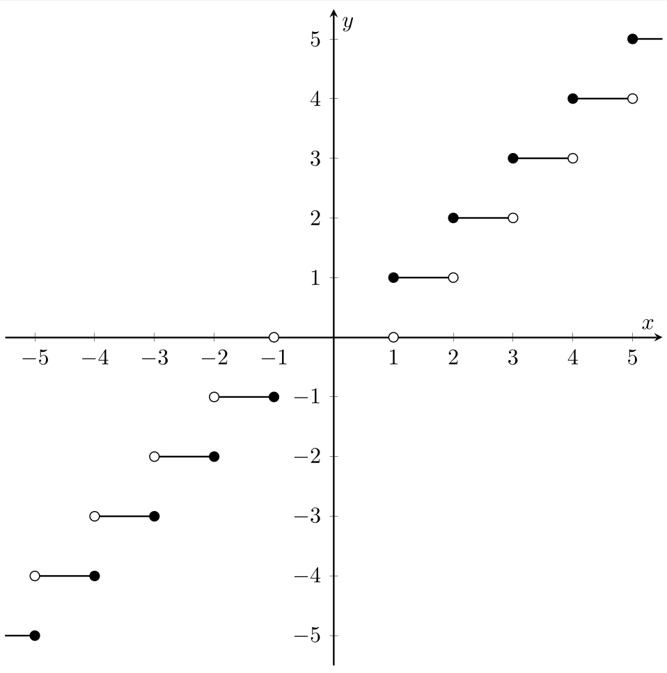
Fig. 2.2 Graph of the function \(g:\mathbb{R}\to\mathbb{R}\); \(g(x)=[x]\) (Problem 8).#
In this case, left and right limits disagree at every \(n \in \mathbb{Z}\setminus\{0\}\). In fact, if \(n\in\mathbb{N}\), then Fig. 2.2 suggests that
At every other real number, the left and right limits exist and are both equal to the value of the function there.
Here some proofs:
To prove \(\lim_{x \rightarrow n^+}[x] = n\): Note that if \(0<x-n<\frac{1}{2}\), we have \([x]=n\), and so \(|[x]-n|=0\). In particular, if \(\varepsilon>0\), then \(0<x-n<\frac{1}{2}\) implies \(|[x]-n|<\varepsilon\).
To prove \(\lim_{x\rightarrow n^-}[x]=n-1\): By the same principle, if \(-\frac{1}{2}<x-n<0\), then \([x]=n-1\), and so \(|[x]-(n-1)|=0\). In particular, for all \(\varepsilon>0\), we have that \(-\frac{1}{2}<x-n<0\) implies \(|[x]-(n-1)|<\varepsilon\).
The proofs of \(\lim_{x\rightarrow -n^+}[x]= -n+1\) and \(\lim_{x\rightarrow -n^-}[x]=-n\) are very similar — or you could just note that \([-x]=-[x]\) and apply algebra of limits.
(iii) We are given \(h:\mathbb{R}\to\mathbb{R}\), \(h(x) =3 - 5\mathbb{1}_{(0, 1]}(x) + 7\mathbb{1}_{(1, 2]}(x)\). Again, it helps to draw a graph first — see Fig. 2.3.
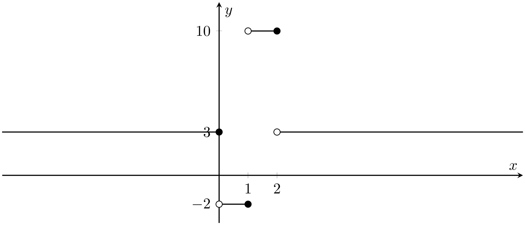
Fig. 2.3 Graph of the function \(h=3 - 5\mathbb{1}_{(0, 1]} + 7\mathbb{1}_{(1, 2]}\) (Problem 8).#
Here, left and right limits disagree at \(x = 0, 1\) and \(2\). We have
To prove \(\lim_{x \rightarrow 0^-}h(x) = 3\) using Definition 2.4, note that for any \(x<0\), \(h(x)=3\) and so \(|h(x)-3|=0\). So for any \(\varepsilon>0\) and any choice of \(\delta>0\), we have that \(-\delta<x<0\) implies \(|h(x)-3|=0<\varepsilon\).
The proof of \(\lim_{x \rightarrow 1^-}h(x) = -2\) is very similar: let \(\varepsilon>0\), and note that if \(-\frac{1}{2}<x-1<0\), then \(\frac{1}{2}<x<1\), and so \(h(x)=-2\). But then, \(|h(x)-(-2)|=0<\varepsilon\).
The proof of \(\lim_{x \rightarrow 2^-}h(x) = 10\) is exactly the same, just take \(-\frac{1}{2}<x-2<0\) and note \(h(x)=10\), instead.
The right limit proofs are similar.
9. (Homework 2 question). The largest subset of \(\mathbb{R}\) for which the formula \(f(x)=\sin\left(\frac{1}{x}\right)\) makes sense is \(A = \mathbb{R} \setminus \{0\}\).
Observe that for any real number \(\theta\in\mathbb{R}\),
To prove \(f\) has no limit at \(0\), we need only choose two values of \(\theta\) for which sine takes distinct values. We choose \(\theta=\frac{\pi}{2}\) and \(\theta=\frac{3\pi}{2}\).
By choosing the right values for \(\theta\), we can use this to construct two distinct sequences \((x_n)\) and \((y_n)\) that both converge to \(0\), but for which \(\sin(x_n)\) and \(\sin(y_n)\) have different limits.
We use \(\theta=\frac{\pi}{2}\) and \(\theta=\frac{3\pi}{2}\) (other choices possible).
For each \(n\in\mathbb{N}\), let \(x_n=\frac{1}{\frac{\pi}{2} + 2\pi n}\) and \(y_n=\frac{1}{3\frac{\pi}{2} + 2\pi n}\). Then
while for all \(n\in\mathbb{N}\),
So \(\lim_{n\rightarrow\infty} f(x_{n}) = 1\), but \(\lim_{n\rightarrow\infty} f(y_n) = -1\). Since these limits are not equal, \(\lim_{x\to 0} f(x)\) does not exist.
Of course, we could have chosen any values of \(\theta\) we liked, and constructed a sequence \((x_n)\) with limit \(0\) for which \(\lim_{n\rightarrow\infty}f(x_n)\) is equal to any real number we liked in the interval \([-1,1]\). The graph of this function (Fig. 2.4) may give some intuition as to how this is possible.
.png)
Fig. 2.4 Graph of the function \(f:\mathbb{R}\to\mathbb{R}\); \(f(x)=\sin\left(\frac{1}{x}\right)\) (Problem 9).#
10. The largest subset of \(\mathbb{R}\) for which the formula \(f(x)=x\sin\left(\frac{1}{x}\right)\) makes sense is \(A = \mathbb{R} \setminus \{0\}\).
We claim that \(\displaystyle\lim_{x \rightarrow 0} x \sin\left(\frac{1}{x}\right) = 0\).
To see this, let \((x_{n})\) be an arbitrary sequence in \(A\) that converges to \(0\). The sine function takes values only in the interval \([-1,1]\), and so
for each \(n\in\mathbb{N}\). Put another way,
for all \(n\in\mathbb{N}\). Since \(\displaystyle\lim_{n\to \infty} x_n=0\), we have \( \displaystyle\lim_{n\to \infty} |x_n| =0\). Therefore, by the squeeze theorem, \(\displaystyle\lim_{n\rightarrow 0}x_n\sin\left(\frac{1}{x_n}\right) = 0\).
Since \((x_n)\) was arbitrary, \(\displaystyle\lim_{x \rightarrow 0} x \sin\left(\frac{1}{x}\right) = 0\).
You should contrast Fig. 2.5 with Fig. 2.4 that for the previous question.
.png)
Fig. 2.5 Graph of the function \(f:\mathbb{R}\to\mathbb{R}\); \(f(x)=x\sin\left(\frac{1}{x}\right)\) (Problem 10).#
11. We’ll just do \(\displaystyle\lim_{x \rightarrow \infty}f(x)\) here, as \(\displaystyle\lim_{x \rightarrow -\infty}f(x)\) is so similar.
(i) Let \(X\subset\mathbb{R}\) and \(f:X\to\mathbb{R}\). We say that \(\lim_{x \rightarrow \infty}f(x) = l\) if for all \(\varepsilon>0\) there exists \(K>0\) such that for all \(x\in X\), \(x>K\) implies \(|f(x)-l|<\varepsilon\).
(ii) The analogue of the sequential criterion is:
\(\lim_{x \rightarrow \infty}f(x) = l\) if for any sequence \((x_{n})\) in \(X\) that diverges to infinity, we have \(\lim_{x \rightarrow \infty}f(x_{n}) = l\).
For the proof, imitate the proof of Theorem 2.1. Suppose the \((\varepsilon- K)\) criterion stated in part (i) holds. Let \(\varepsilon>0\), and choose \(K>0\) such that for all \(x\in X\), \(x>K\) implies \(|f(x)-l|<\varepsilon\). Let \((x_n)\) be any sequence in \(X\) that diverges to infinity. Then using the same \(K>0\), there exists \(N\in\mathbb{N}\) such that if \(n\geq N\), then \(x_{n} > K\). But then, for all \(n\geq N\), \(x_n>K\), which in turn implies \(|f(x_{n}) - l| < \varepsilon\). Hence \(\lim_{x \rightarrow \infty}f(x_{n}) = l\), as required.
For the converse, we prove by contrapositive. Suppose the \((\varepsilon-K)\) criterion does not hold. Then there exists \(\varepsilon>0\) such that for all \(K>0\), there is \(x\in X\) for which \(x>K\) and \(|f(x)-l|\geq \varepsilon\). Apply this successively to \(K = 1, 2, 3, \ldots\). For \(K=n\), we get \(x_n\in X\) with \(x_{n} > n\), and \(|f(x_{n}) - l| \geq \varepsilon\) for each \(n\in\mathbb{N}\). But then, \((x_n)\) is a sequence in \(X\) diverging to infinity, and such that \(f(x_n)\nrightarrow l\). This shows that the sequential criterion fails.
(iii) Using the definition: Given any \(\varepsilon > 0\), choose \(K = \frac{1}{\varepsilon}\). Then \(x > K \Rightarrow \frac{1}{x} < \varepsilon\), and so \(\lim_{x\to\infty} \frac{1}{x}=0\).
Using sequences: Let \((x_n)\) be any sequence in \(\mathbb{R}\setminus\{0\}\) diverging to infinity as \(n\rightarrow\infty\). Then, by algebra of limits, \(\frac{1}{x_n}\rightarrow 0\). Since the sequence was chosen arbitrarily, it follows that \(\lim_{x\rightarrow\infty}\frac{1}{x}=0\).
The case where \(x\to-\infty\) is similar.
12. (i) Let \(f:X\to\mathbb{R}\) be a function, where \(X\subseteq\mathbb{R}\). We say that \(\lim_{x \rightarrow \infty} f(x) = \infty\) if:
Given any \(M > 0\), there exists \(K > 0\) such that \(x > K\) implies \(f(x) > M\).
The analogue of the sequential criterion is:
For any sequence \((x_{n})\) in \(X\) which diverges to infinity, we also have that \((f(x_{n}))\) diverges to infinity.
The other cases are similar.
(ii) Let \(f:\mathbb{R}\to[0,\infty)\), \(g:\mathbb{R}\to[0,\infty)\), and suppose \(\displaystyle\lim_{x\rightarrow\infty}f(x)=\infty\) and \(\displaystyle\lim_{x\rightarrow\infty}g(x)=l\), where \(l>0\).
Let \(M > 0\). Since \(\lim_{x\rightarrow\infty}f(x)=\infty\), there exists \(K_1 > 0\) such that
Since \(\lim_{x\rightarrow\infty}g(x)=l\), for all \(\varepsilon>0\) we can find \(K_2>0\) such that \(x>K_2\) implies \(|g(x)-l|<\varepsilon\). In other words,
This is true for all \(\varepsilon\). We apply it specifically to \(\varepsilon = \frac{l}{2}\). Then, there is \(K_2>0\) such that
Let \(K=\max\{K_1,K_2\}\). If \(x>K\), then \(x>K_1\) and \(x>K_2\), so \(f(x)>\frac{2M}{l}\) and \(\frac{l}{2} < g(x) < \frac{3l}{2}\).
Hence for \(x>K\),
That is, \(\lim_{x\rightarrow\infty}f(x)g(x) = \infty\).
(iii) Let \(p:\mathbb{R}\to\mathbb{R}\) be a polynomial of even degree \(m\), with positive leading coefficient. Write \(m = 2n\) and let
We use part (ii). Take \(f(x) = x^{2n}\) and \(\displaystyle g(x) = a_{2n} + \frac{a_{2n-1}}{x} + \cdots + \frac{a_{1}}{x^{2n-1}} + \frac{a_{0}}{x^{2n}}\).
Observe that \(\displaystyle\lim_{x \rightarrow \infty}f(x) = \infty\) and \(\displaystyle\lim_{x \rightarrow \infty}g(x) = a_{2n}\). Hence by part (ii),
If \(n\) is odd, \(\lim_{x \rightarrow \infty}p(x) = \infty\), but \(\lim_{x \rightarrow -\infty}p(x) = -\infty\).
2.3. Continuity#
13. For each of (i) to (v), the function is continuous at each point of its domain. For (i), (ii) and (iii), we have rational functions, which are continuous on all points of \(A\) (which is the subset of \(\mathbb{R}\) where the denominator is non-zero). For (iv) and (v), we have compositions of rational functions with the exponential and cosine functions, which are continuous on the whole of \(\mathbb{R}\). Again, the functions are continuous on all points of \(A\) (which is the subset of \(\mathbb{R}\) where the denominator of the rational function is non-zero).
14. If \((x_{n})\) is any sequence that converges to \(a\), we know that \(f(x_n)\) converges to \(f(a)\) as \(f\) is continuous at \(a\), and we need to show that \((|f|(x_n))\) converges to \(|f|(a)\).
By Corollary 1.1, if \((x_{n})\) is any sequence that converges to \(a\),
as \(f\) is continuous. So by the squeeze theorem, \(\lim_{n\rightarrow\infty} |f|(x_{n}) = |f|(a)\), and so \(f\) is continuous at \(a\).
15. Let \((x_{n})\) be a sequence in \(A\) that converges to \(a\). Since \(f\) is continuous at \(a\) we have \(\lim_{n\rightarrow\infty} f(x_{n}) = f(a)\). And then, since \(g\) is continuous at \(f(a)\), we have \(\lim_{n\rightarrow\infty} g(f(x_{n})) = g(f(a))\), and the result follows.
16. \(f \circ g:\mathbb{R}\to \mathbb{R}\) given by \((f \circ g)(x) = \frac{1}{1 + x^{2}}\). It is continuous on \(\mathbb{R}\) by Theorem 3.2(iv).
\(g \circ f:\mathbb{R} \setminus \{0\} \to \mathbb{R} \setminus \{0\}\) given by \((g \circ f)(x) = {1 + \frac{1}{x^2}}\). It is continuous on \(\mathbb{R} \setminus \{0\}\) by Theorem 3.2(iv).
17. The proofs for each of these answers are immediate by Problem 8.
(i) \(f:\mathbb{R}\to\mathbb{R}\); \(f(x) = \begin{cases} 1 -x & \text{if }x < 1\\ x^{2}& \text{if }x \geq 1. \end{cases}\)
This function is continuous on \(\mathbb{R} \setminus \{1\}\), with a jump discontinuity at \(x=1\) of size \(1\).
(ii) \(g:\mathbb{R}\to\mathbb{R}\); \(g(x) = [x] = \left\{\begin{array}{cl} \lfloor x\rfloor & \text{ if } x\geq 0 \\ \lceil x \rceil & \text{ if } x<0 \end{array}\right.\)
This function is continuous on \(\mathbb{R}\setminus\{\pm k: k\in\mathbb{N}\}\). Jump discontinuity at \(n\) with size \(1\) for all \(n\in\mathbb{Z}_+\).
(iii) \(h:\mathbb{R}\to\mathbb{R}\); \(h(x) =3 - 5\mathbb{1}_{(0, 1]}(x) + 7\mathbb{1}_{(1, 2]}(x)\)
This is continuous at \(\mathbb{R} \setminus \{0,1,2\}\), with jump discontinuities at \(0\), \(1\), and \(2\). The jump sizes are, respectively, \(0\), \(-5\), and \(-7\).
18. (Homework 3 question).
(i) We are given \(f:\mathbb{R} \setminus \{0\} \rightarrow \mathbb{R}\); \(f(x) = \frac{(1 + x)^{2} - 1}{x}\), a continuous function (since it is a rational function).
For \(x \neq 0, f(x) = x+2\), and so \(\lim_{x \rightarrow 0}f(x) = 2\), by algebra of limits. Therefore the required continuous extension of \(f\) is
Or, put more simply: \(\tilde{f}(x)=x+2\) for all \(x\in\mathbb{R}\).
(ii) Let now \(f(x) = \frac{(x-2)(x^{2} + 2x + 4)}{(x-2)(x+2)}\). The largest possible domain for \(f\) is \(A=\mathbb{R} \setminus \{-2, 2\}\) (the set where the denominator is non-zero). For \(x \neq 2, -2\),
This is a rational function, and hence continuous everywhere the denominator is non-zero by Theorem 3.2(iv).
We claim that \(\lim_{x \rightarrow -2}f(x)\) does not exist. To see this, consider the sequence \((x_{n})\) given by \(x_n=-2 + \frac{1}{n}\). Then,
Thus \(f\) has no continuous extension to the point \(x =-2\).
[Note: Here, we have proven that \(f(x)\) does not converge as \(x\rightarrow-2\). We have not proven that \(\lim_{x\rightarrow -2} f(x)=-\infty\). To show this, we would have had to choose an arbitrary sequence \((x_n)\) in \(A\) with limit \(-2\) and proven that for this general sequence, \(\lim_{n\rightarrow\infty}f(x_n)=-\infty\) (or constructed an \(K-\delta\) argument using Definition 2.3). ]
On the other hand, \(f\) does have a continuous extension to \(\mathbb{R}\setminus\{-2\}\). Indeed, by algebra of limits we have
and so \(f\) has a continuous extension
We can see this behaviour in the graph of the function (Fig. 2.6)
,(x+2).png)
Fig. 2.6 Graph of the function \(\tilde{f}:\mathbb{R}\setminus\{-2\}\to\mathbb{R}\); \(f(x)=x+\frac{4}{x+2}\) (Problem 18).#
19. (Homework 2 question). Assume \(g\) is continuous and \(g(a) > 0\). Then for all \(\varepsilon>0\) there exists \(\delta>0\) such that for all \(x\in\mathbb{R}\), \(|x-a|<\delta\) implies \(|g(x)-g(a)|<\varepsilon\). Let \(\varepsilon=\frac{g(a)}{2}\). Then for some \(\delta>0\), we have \(|g(x)-g(a)|<\frac{g(a)}{2}\). But then \(\frac{g(a)}{2}<g(x)<\frac{3g(a)}{2}\), and in particular, \(g(x)>\frac{g(a)}{2}>0\).
Alternate solution using sequences:
Suppose, for a contradiction, that there is no \(\delta > 0\) such that \(g(x) > 0\) for all \( x \in (a - \delta, a + \delta)\). Then, in particular, for all \(n\in\mathbb{N}\) there exists \(x_{n} \in \left(a - \frac{1}{n}, a + \frac{1}{n}\right)\) such that \(g(x_{n}) \leq 0\). By the squeeze theorem, we have \(\lim_{n\rightarrow\infty} x_{n} = a\). So, by continuity of \(g\) at \(a\), we have \(\lim_{n\rightarrow\infty} g(x_{n})\) exists and equals \(g(a)\). But \(g(x_n)\leq 0\) for all \(n\in\mathbb{N}\), and so
which is a contradiction.
20. (i)
On the other hand,
and the result follows.
Then for all \(x \in A\cap B,\)
and continuity follows by Theorem 3.2(i) and (iii) and Problem 14.
(ii) You can check that for all \(a, b \in \mathbb{R}\),
and then argue as in (i).
Alternatively, one could derive (ii) from (i) by using \(\min\{f,g\} = - \max\{-f, -g\}\).
21. Let \(f: \mathbb{R} \rightarrow \mathbb{R}\) be such that
Then:
(i) \(f(0) = f(0 + 0) = f(0) + f(0) = 2f(0)\), hence \(f(0) = 0\).
(ii) For all \(x\in\mathbb{R}\), we have by (i), \(0 = f(0) = f(x + -x) = f(x) + f(-x)\). So \(f(-x)=-f(x)\).
(iii) Suppose \(f\) is continuous at zero. Then, if \(x \neq 0\) then any sequence \((x_{n})\) which converges to \(x\) can be written as \(x_{n} = x + y_{n}\) where \((y_{n})\) converges to zero. Since \(f\) is assumed to be continuous at \(0\), we have that \( \lim_{n\rightarrow\infty} f(y_{n})\) exists and equals \(f(0)\). By (i), \(f(0)=0\), hence
(iv) Let \(k=f(1)\). We use induction on \(n\in\mathbb{N}\). If \(n=1\), then \(f(n)=f(1)=k=k\cdot 1\), so the statement holds. Assume it holds for some \(n\in\mathbb{N}\). Then by (2.2),
Hence by induction, \(f(n)=nk\), for all \(n\in\mathbb{N}\). Combine this with part (ii) to extend to all \(n\in \mathbb{Z}\).
(v) Still writing \(k=f(1)\), consider \(\frac{p}{q}\in\mathbb{Q}\), where \(p\in \mathbb{Z}\) and \(q\in \mathbb{N}\). By (iv),
and the result follows.
(vi) Finally, let \(k=f(1)\), and assume \(f\) is continuous at \(0\), and let \(x\in\mathbb{R}\). If \(x\in\mathbb{Q}\), then we have already shown \(f(x)=kx\) in part (v). So assume \(x\) is irrational. By denseness of the rationals, there is a sequence \((r_n)\) of rational numbers converging to \(x\). By (v), \(f(r_n)=kr_n\) for all \(n\in\mathbb{N}\). By (iii), \(f\) is continuous at \(x\), so using algebra of limits, we have
22. (Homework 2 question). Recall from Example 3.10 in the notes that Dirichlet’s “other” function (AKA Thomae’s function) is defined \(g:[0, 1)\rightarrow \mathbb{R}\) defined by
Suppose that \(a \in \mathbb{Q}\cap[0,1)\). Then \(g(a)=\frac{1}{k}\), for some fixed \(k\in\mathbb{N}\). Every real number is the limit of a sequence of irrational numbers[1]. Therefore, there is a sequence \((x_{n})\) of irrational numbers that converges to \(a\). Since \(a\in[0,1)\), we may assume (removing some initial terms if necessary) that \(x_n\in[0,1)\setminus\mathbb{Q}\) for all \(n\in\mathbb{N}\).
If \(g\) was continuous at \(a\), we would have \(\lim_{n\rightarrow\infty}g(x_n)=g(a)\). But in fact, \(g(x_n)=0\) for all \(n\in\mathbb{N}\), so \(\lim_{n\rightarrow\infty}g(x_n)=0\neq \frac{1}{k}=g(a)\).
It follows that \(g\) is discontinuous at every rational point of its domain.
23. The function \(\mathbb{1}_{(a, b)}\) is left continuous at \(a\) (but not right continuous), and right continuous at \(b\) (but not left continuous).
To prove the left continuity at \(a\), let \((x_{n})\) be any sequence in \(\mathbb{R}\) which converges to \(a\) with \(x_{n} < a\) for all \(n\in\mathbb{N}\). Then \(\lim_{n\rightarrow\infty} \mathbb{1}_{(a, b)}(x_{n}) = 0 = \mathbb{1}_{(a, b)}(a).\) On the other hand to see that it is not right continuous at \(a\), let \((y_{n})\) be any sequence in \(\mathbb{R}\) which converges to \(a\) with \(a < y_{n} < b\) for all \(n\in\mathbb{N}\). Then
\( \lim_{n\rightarrow\infty} \mathbb{1}_{(a, b)}(y_{n}) = 1 \neq \mathbb{1}_{(a, b)}(a). \) The other assertion is proved similarly.
[Contrast this with \(\mathbb{1}_{[a, b]}\), which was discussed in the notes.]
24. Since \(f\) is continuous on \([a, b]\), so is \(g\). We have \(g(a) = f(a) - \gamma < 0\) and \(g(b) = f(b) - \gamma > 0\). Hence by Proposition 3.1, there exists \(c \in (a, b)\) with \(g(c) = 0\), i.e. \(f(c) = \gamma\), as was required.
25. (Homework 3 question). Let \(a,b\in\mathbb{R}\), \(a<b\), and suppose \(f:[a,b] \rightarrow (a,b)\) is a continuous function.
The question suggests we consider a function of the form \(g(x) = f(x) - \) (something), and apply the intermediate value theorem. Since we seek a point \(c\in(a,b)\) for which \(f(c)=c\), we try \(g(x)=f(x)-x\). This is a continuous function on \([a,b]\), since \(f\) is. Moreover, any zero of \(g\) will be a fixed point of \(f\).
Since the range of \(f\) is contained in \((a, b)\), we have \(a<f(x)<b\) for all \(x\in[a,b]\). In particular, \(f(a) > a\) and \(f(b) < b\), and so \(g(a) = f(a) - a > 0\) and \(g(b) = f(b) - b < 0\). In other words, \(0\in(g(a),g(b))\). By the intermediate value theorem (or by Proposition 3.1, the special case where \(\gamma=0\)), there exists \(c \in (a, b)\) such that \(g(c) = 0\), i.e., such that \(f(c) = c\).
For the counter–example, consider \(f:(0,1)\to(0,1)\), \(f(x) = x^2\). It is continuous on \((0, 1)\) but there is no \(c \in (0, 1)\) for which \(c^2 = c\).
26. Define \(\gamma = \inf_{x \in [a, b]}f(x)\) and assume that it is not attained, so \(\gamma < f(x)\) for all \(x \in [a,b]\). Then consider the function
This is continuous, and hence bounded on \([a, b]\). So there exists \(K \geq 0\) such that \(|h(x)| \leq K\) for all \(x \in [a, b]\). Since \(\gamma=\inf_{x\in[a,b]}f(x)\), given any \(\varepsilon > 0\), there exists \(x \in [a, b]\) such that \(f(x) < \gamma + \varepsilon\). Now take \(\varepsilon = \frac{1}{K}\) to deduce that \(h(x) > K\), which yields the required contradiction.
[Alternatively: We proved in lectures that continuous functions on \([a,b]\) are bounded and attain a maximum value. Since \(f\) is continuous on \([a,b]\), so is \(-f\), and hence \(-f\) attains a maximum: say \(k\in[a,b]\) is such that \(-f(k)=\sup_{x\in[a,b]}(-f(x))\). Then, using a standard property[2] of sup’s and inf’s,
In other words, \(f\) attains its minimum.]
27. (i) Let \(f:\mathbb{R}\to\mathbb{Z}\) be continuous, and suppose \(f\) is not a constant function.
Then there must be \(a,b\in\mathbb{R}\) such that \(a\neq b\) and \(f(a)\neq f(b)\). Without loss of generality, assume \(a<b\).
Then \(f\) is continuous on \([a,b]\), and since \(f(a)\neq f(b)\), \(f\) is also non-constant on \([a,b]\). By Corollary 3.3, \(f([a,b]])=[m,M]\). This contradicts \(f\) having codeomain \(\mathbb{Z}\).
It follows that \(f\) must be a constant function.
(ii) Argue as in (i), using the fact that between any two rational numbers, we can find an irrational number.
28. By algebra of limits, \(\frac{1}{f}\) is continuous on \([0, 1]\) and so is bounded by Theorem 3.5.
29.
If \(f\) is continuous on \([0, 1]\), then it is bounded by Theorem 3.5, and so there exists \(L \geq 0\) such that \(|f(x)| \leq L\) for all \(x \in [0, 1]\). Hence the range of \(f\) is a subset of \([-L, L]\) and cannot be all of \(\mathbb{R}\).
30. Since \((x_{n})\) is bounded, by the Bolzano–Weierstrass theorem it has a convergent subsequence \((x_{n_{k}})\). Let \(c=\lim_{k \rightarrow \infty}x_{n_{k}}\) and note that \(c \in [0, 1]\), since \(x_{n_k}\in[0,1]\) for all \(k\).
A straight-forward induction argument shows that \(f(x_{n_{k}}) \leq r^{n_{k}-1}f(x_{n_{1}})\) for all \(k\in\mathbb{N}\). But then, since the range of \(f\) is contained in \([0,1]\), we have
for all \(k\in\mathbb{N}\). Since \(r < 1\), \(\lim_{k\to\infty} r^{n_k-1} =0\). By the squeeze theorem, \( \lim_{k \rightarrow \infty}f(x_{n_{k}}) = 0\) and by continuity of \(f\) at \(c\), \(f(c) = \lim_{k \rightarrow \infty}f(x_{n_{k}})\), so \(f(c)=0\).
31. For all \(x > y\),
32. For all \(-\frac{\pi}{2} \leq x < y \leq \frac{\pi}{2}\),
so the function is strictly monotonic increasing on this interval. It is also continuous (stated in notes), and so by Theorem 3.6, it is has a continuous inverse \(f^{-1}(x) = \arcsin(x)\) (or \(\sin^{-1}(x)\)) defined on \([-1, 1]\). Outside the interval \(\left[-\frac{\pi}{2}, \frac{\pi}{2}\right]\), the function \(f\) might fail to be strictly increasing. In fact it is strictly decreasing on each interval of the form \(\left((4n+1)\frac{\pi}{2}, (4n + 3)\frac{\pi}{2}\right)\), and strictly increasing on each interval of the form \(\left((4n-1)\frac{\pi}{2}, (4n + 1)\frac{\pi}{2}\right)\), where \(n\in\mathbb{Z}_+\).
33. We seek a continuous extension of the mapping \(x\mapsto \frac{1-x}{1-x^{\frac{m}{n}}}\) to a domain that includes \(1\). Then, we can use continuity to evaluate the limit as \(x\rightarrow 1\).
Observe that, if we write \(y = x^{\frac{1}{n}}\), then
by the geometric sum formula. Note that the left hand side is not defined at \(x=1\), but the right hand side is.
Let \(f:[0,\infty)\to[0,\infty)\); \(f(x)=x^{\frac{1}{n}}\), and let
Both \(f\) and \(g\) are continuous at every point in their domain (for \(f\), this was proven in Example 3.9). Hence by the composition theorem for continuous functions (Theorem 3.3), the map
is continuous. Also, by our initial calculation,
whenever \(x\geq 0\) and \(x^{\frac{m}{n}}\neq 1\). Therefore,
by continuity of \(g\circ f\).
34. We claim that if \(a < x < b\), we have \(f(a) < f(x) < f(b)\). To see this, note that if \(f(a) \geq f(x)\) then either \(f(a) = f(x)\), or \(f(a) > f(x)\).
If \(f(a)=f(x)\), then \(f\) cannot be bijective, which is a contradiction.
Suppose that \(f(a)>f(x)\). Applying Corollary 3.3 to \(f|_{[x,b]}\), the image of \([x,b]\) under \(f\) must an interval, \([m,M]\), say. Note that \(f(a)\in(m,M)\): indeed, \(f(a)>f(x)>M\), and \(f(a)<f(b)<m\). Therefore, by the intermediate value theorem (or Corollary 3.1 more specifically), there exists \(c \in (x, b)\) such that \(f(c) = f(a)\), and this again violates the injectivity of the mapping \(f\). A similar argument can be used to show that we cannot have \(f(b) \leq f(x)\).
Finally, applying our initial result to \(f|_{[a, y]}\), we see that if \(a<x<y<b\), then \(f(a) < f(x) < f(y)\). Hence \(f\) is strictly monotonic increasing.
35.* First observe that \(f+g\) is monotonic increasing since both \(f\) and \(g\) are. Choose \(a \in \mathbb{R}\). Given \(\varepsilon > 0\), there exists \(\delta > 0\) so that if \(x > a + \delta\) then
and so
as \(g\) is increasing. This proves that \(g\) is right–continuous at \(a\). A similar argument (interchanging the roles of \(a\) and \(x\)) proves that it is left–continuous, and hence continuous at \(a\). Then \(g = (f + g) - f\) is the difference of two continuous functions, and hence is itself continuous.
36.*
(i) If \(0<a<1\), then \(0<a<\sqrt{a}<1\). So \((x_n)\) is monotonic increasing and bounded above by \(1\), and hence converges to some limit \(0\leq l\leq 1\). By continuity of the square root function, \(\sqrt{l}=\lim_{n\rightarrow\infty}\sqrt{x_n}\). But \(\sqrt{x_n}=x_{n+1}\rightarrow l\) as \(n\rightarrow\infty\). By uniqueness of limits, \(\sqrt{l}=l\), and so \(l=1\).
If instead \(a>1\), then \(a>\sqrt{a}>1\), and so \((x_n)\) is monotonic decreasing and bounded below by \(1\). So the sequences converges to a limit, and by an identical argument to above, this limit has to be \(1\).
(ii) For all \(a>0, n\in\mathbb{N}, f(a) = f\left(a^{\frac{1}{2}}\right) = \cdots = f\left(a^{\frac{1}{2^{n-1}}}\right)\). That is, \(f(a)=f(x_n)\) for all \(n\in\mathbb{N}\). By continuity,
If \(a<0\), then \(a^2>0\) and so \(f(a)=f\left(a^2\right)=f(1)\). Finally, by continuity,
and we have shown that \(f(x)=f(1)\) for all \(x\in\mathbb{R}\).
2.4. Differentiation#
37. This is Definition 2.2 in the notes:
The function \(f\) has limit \(l\) at the point \(a\) if for every \(\varepsilon>0\) there exists \(\delta>0\) such that for all \(x\in X\),
We write \(\lim_{x\to a}f(x)=l\).
(i) This is Definition 4.1 in the notes: we say that \(f\) is differentiable at \(a \in A\) if \( \lim_{x \rightarrow a}\frac{f(x) - f(a)}{x - a}\) exists. Or, equivalently, \( \lim_{h \rightarrow 0}\frac{f(a +h) - f(a)}{h}\) exists.
That is, we fix \(a\in A\) and we consider the function \(g\) given by \(g(h)=\frac{f(a +h) - f(a)}{h}\). Then \(f\) is differentiable at \(a\) if the limit of \(g\) as \(h\) goes to zero exists.
(ii) Using the sequential criterion (Theorem 2.1 in the notes):
\(f\) is differentiable at \(a\) if there exists some number \(f'(a) \in \mathbb{R}\) for which, given any sequence \((h_{n})\) that converges to \(0\), with \(h_n\neq 0\) for all \(n\), we have
(iii) This is asking for the equivalent description of limit of a function given by the \((\varepsilon - \delta)\) criterion (Theorem 2.1). Again it needs to be applied to \(g\) as above not \(f\) itself:
We say \(f\) is differentiable at \(a\) if there exists a number \(f'(a)\) for which, given \(\varepsilon>0\), there exists \(\delta > 0\) such that if \(0<|h| < \delta\), then
39. Let \(x\in\mathbb{R}\setminus\{0\}\). Then
Thus \(f\) is differentiable at all \(x\in\mathbb{R}\setminus\{0\}\) and \(f'(x)=-\frac{1}{x^2}\) for all \(x\in\mathbb{R}\setminus\{0\}\).
The extended function (where we define its value at \(x=0\) to be zero) is not continuous at \(x=0\), since \(\lim_{x \rightarrow 0^+}\frac{1}{x} =\infty\). Therefore it is not differentiable at \(x=0\), by Theorem 4.1.
40. As in the hint, let \(g(h) = e^{kh} - 1 - kh \). Then
using the given fact that \(\lim_{h \rightarrow 0}\frac{g(h)}{h} = 0\). Thus \(f\) is differentiable at each \(x\in\mathbb{R}\) and \(f'(x)=ke^{kx}\).
41. (Homework 5 question).
(i) Using the product and chain rules for differentiation, and that \(\sin\) is differentiable with derivative \(\cos\), if \(x \neq 0\), \(f\) is differentiable at \(x\) with \(f'(x) = \sin\left(\frac{1}{x}\right) - \frac{1}{x}\cos\left(\frac{1}{x}\right)\).
(ii) But \(\frac{f(x) - f(0)}{x} = \sin\left(\frac{1}{x}\right)\) has no limit as \(x \rightarrow 0\) (see Problem 9), so \(f\) is not differentiable at \(0\).
42. Let \(f:\mathbb{R}\to \mathbb{R}\) given by
Using the product and chain rules and standard derivatives, for \(x \neq 0\), \(f\) is differentiable at \(x\) with \(f'(x) = 2x\sin\left(\frac{1}{x}\right) - \cos\left(\frac{1}{x}\right)\). At \(x = 0,\)
by Problem 10. So \(f\) is differentiable at \(0\) with \(f'(0) = 0\). For the second derivative, with \(x \neq 0\), we have
But \(f^{\prime \prime}\) doesn’t exist at \(x = 0\), as in Problem 41.
43. We give sketches of simple examples of functions as described. There should be some kind of “corner” or “cusp” at the relevant points, so that there is clearly no well-defined gradient there. But the functions are required to be continuous, so there should be no jump or other discontinuity.
(i) Fig. 2.7
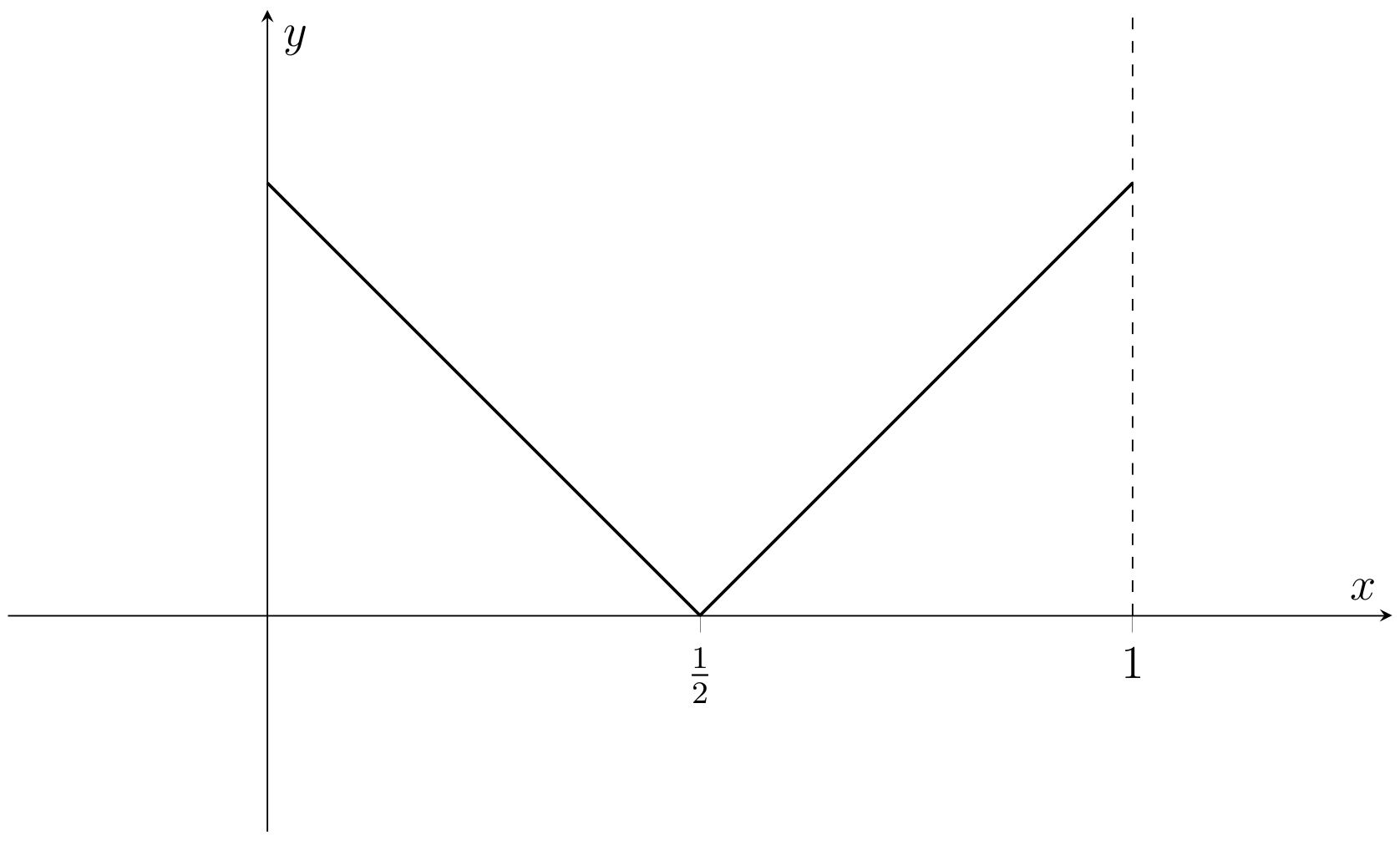
Fig. 2.7 Graph of a function \(f:[0,1]\to\mathbb{R}\) that is not differentiable at \(\frac{1}{2}\), but is everywhere else (Problem 43(i)).#
(ii) Fig. 2.8
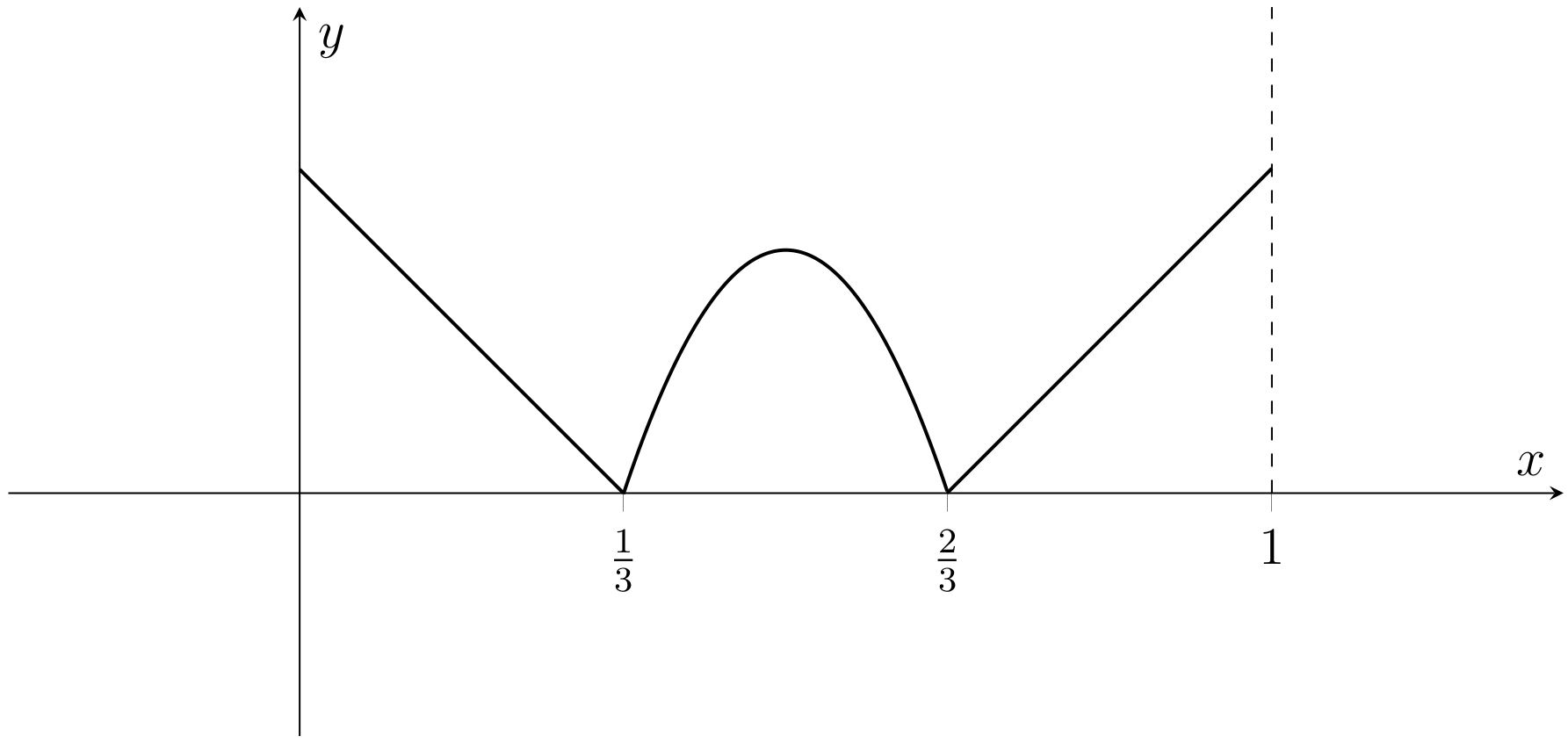
Fig. 2.8 Graph of a function \(f:[0,1]\to\mathbb{R}\) that is differentiable at all points in its domain apart from \(\frac{1}{3}\) and \(\frac{2}{3}\) (Problem 43(ii)).#
44. It helps to sketch the graph. On the interval \([0,1]\), we have \([x]=0\) and so the graph resembles \(y=x\). This pattern then repeats, and we have the following graph for \(f(x)=x-[x]\) — see Fig. 2.9
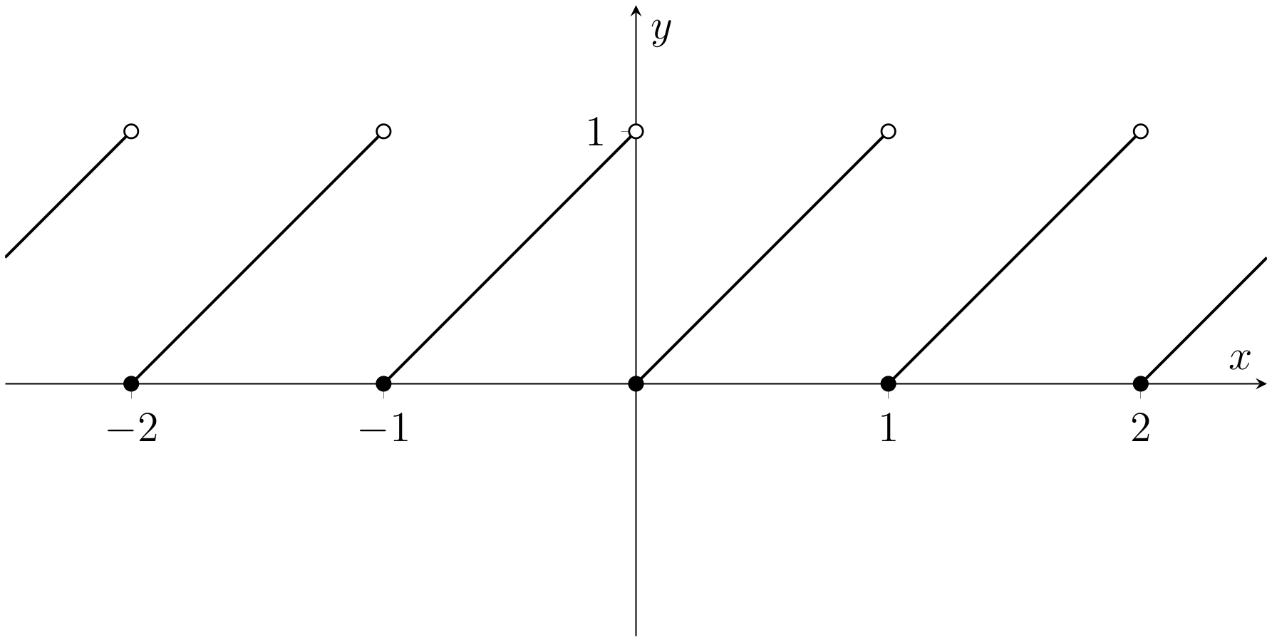
Fig. 2.9 Graph of the function \(f:\mathbb{R}\to\mathbb{R}\); \(f(x)=x-[x]\) (Problem 44).#
The function \(f\) is differentiable for all \(x \in \mathbb{R} \setminus \mathbb{Z}\). For such points, taking \(h>0\) sufficiently small, we have \([x+h]=[x]\) and so
Thus \(f'(x) = 1\) for all \(x \in \mathbb{R} \setminus \mathbb{Z}\). If \(x \in \mathbb{Z}\), then \(f\) is not continuous at \(x\) (it has a jump discontinuity of \(-1\) there) and so cannot be differentiable there (by Theorem 4.1).
45. First observe that if \(f\) is differentiable at \(a\), then
So
On the other hand, by Example 5.2.5, \(f:\mathbb{R}\to\mathbb{R}\) given by \(f(x)=|x|\) is not differentiable at \(x=0\). But
46. (i) True: \(f\) is continuous at zero as \(f(0) = 0= \lim_{x \rightarrow 0^-}f(x) = \lim_{x \rightarrow 0^+}f(x)\).
(ii) True: \(f'(0)\) exists and is zero. To see this compute
and
(iii) True: \(f'\) is continuous at zero since \(f':\mathbb{R}\to\mathbb{R}\) is given by
so \(f'(0) = \lim_{x \rightarrow 0^-} f'(x) = \lim_{x \rightarrow 0^+}f'(x) = 0\).
(iv) False: \(f^{\prime \prime}_{+}(0) = \lim_{h \rightarrow 0^+}\frac{2h - 0}{h} = 2, f^{\prime \prime}_{-}(0) = \lim_{h \rightarrow 0^-}\frac{-2h - 0}{h} = -2\), and so \(f^{\prime \prime}(0)\) does not exist.
47. 47. (Homework 5 question).
(i) Yes: \(f\) is differentiable on \([a, b]\) and hence continuous on \([a, b]\) by Theorem 4.1, so it attains its sup and inf on \([a, b]\) by the extreme value theorem, Theorem 3.5, and these are the maximum and minimum (respectively).
(ii) No: the maximum or minimum could be \(f(a)=f(b)\). If \(f(a)\) is not the maximum value, then this must occur in \((a, b)\). Similarly for the minimum. If \(f(a) = f(b)\) is both the maximum and minimum value, then \(f\) is constant, and the value occurs in \((a, b)\).
48. Following the hint, define \(g:\mathbb{R}\rightarrow \mathbb{R}\) by
Then \(g\) is a polynomial, so it is differentiable on \([0, 1]\) and using standard derivatives, \(g'(x)=f(x)\). Also \(g(0) = g(1) = 0\). So by Rolle’s theorem, there exists \(c \in (0, 1)\) such that \(g'(c) = 0\), i.e.\(f(c) = 0\).
49. (i) Let \(x, y\) be such that \(a \leq x < y \leq b\). We want to show that \(f(x)=f(y)\).
Apply the mean value theorem to the restriction of \(f\) to the interval \([x, y]\), to find there exists \(d \in (x, y)\) for which
By assumption, \(f'(c)=0\) for all \(c\in(a,b)\), so \(f'(d)=0\).
Thus \(f(x)=f(y)\). Since this holds for all \(x,y\in [a,b]\), \(f\) is constant on \([a,b]\).
(ii) Define \(f:\mathbb{R}\to\mathbb{R}\) by \(f = h-g\). Then the function \(f\) is continuous on \([a,b]\) and differentiable on \((a,b)\), because \(g\) and \(h\) are, and \(f'(x)=h'(x)-g'(x)=0\) for all \(x\in (a,b)\). Thus \(f\) satisfies all the conditions of (i). By part (i), \(f\) is constant on \([a,b]\). That is, there exists some \(k\in \mathbb{R}\), such that \(f(x)=k\) for all \(x\in [a,b]\). Thus \(h(x)=g(x)+k\) for all \(x\in [a,b]\).
50. By the mean value theorem, \(f(b) = f(a) + f'(c)(b - a)\) for some \(c\in (a,b)\). So, since \(m \leq f'(c) \leq M\), for all \(c \in (a, b)\),
51. The polynomial \(p\) is of odd degree so it has at least one real root by Example 3.12. Also \(p\) is differentiable with \(p'(x) = 3x^{2} + r > 0\), for all \(x \in \mathbb{R}\), so \(p\) is strictly monotonic increasing on any closed interval \([a, b]\), and hence on the whole of \(\mathbb{R}\), by Corollary 4.1. Then by the inverse function theorem (Theorem 3.6), \(p\) is invertible and hence injective, and so there is exactly one zero.
52. Let \(r>1\) and fix \(y\in (0,1)\). Apply the mean value theorem to the function \(f:[y,1]\to\mathbb{R}\) given by \(f(x) = x^r\). Then there exists \(c \in (y, 1)\) such that
Now, \(0<c<1\), and \(r>1\), so \(c^{r-1}<1\). Thus
53. Consider the first case. Here we have
In particular, \(f^{\prime \prime}_{+}(a) = \lim_{h \rightarrow 0^+}\frac{f'(a + h)}{h} < 0\), and so \(f'(a + h) < 0\) for sufficiently small positive \(h\), (say \(0 < h < \delta\)), in which case, by Corollary 4.1, \(f\) is strictly decreasing on \([a, a + \delta]\). We also have \(f^{\prime \prime}_{-}(a) = \lim_{h \rightarrow 0^-}\frac{f'(a + h)}{h} < 0\), and so \(f'(a + h) > 0\) for sufficiently small negative \(h\), (say \(-\delta_{1} < h < 0\)), in which case, by Corollary 4.1, \(f\) is strictly increasing on \([a- \delta_{1}, a]\). Then it follows that \(f\) has a local minimum at \(a\). The other case is similar.
2.5. Sequences and series of functions — Non-examinable 2024–25#
54. For \(x\in [0,\pi ]\) we have \(0\leq \sin x<1\) except when \(x=\frac{\pi}{2}\), where \(\sin x=1\). Thus \(f_n(x)\) converges pointwise to the function \(f\colon [0, \pi ]\rightarrow \mathbb{R}\) defined by
Each function \(f_n\) is continuous. The function \(f\) is not continuous. So the sequence \((f_n)\) does not converge uniformly (otherwise we would have a contradiction to Theorem 5.1 — the uniform limit theorem).
55. (i) Observe that \((f_n)\) converges pointwise to the function
Each function \((f_n)\) is continuous, but the function \(f\) is not continuous at \(0\), so the convergence cannot be uniform.
(ii) Let \(x\in \mathbb{R}\). Then for any \(n\geq x\), we have \(f_n (x) =0\), so the sequence \((f_n)\) converges pointwise to the zero function.
On the other hand
so certainly \((M_n)\) does not converge to zero, and the sequence \((f_n)\) therefore does not converge uniformly to the zero function.
(iii) For \(x>1\), \(\frac{1}{x^n} \rightarrow 0\) as \(n\rightarrow \infty\). Hence for each \(x\in (1,\infty )\), \(\frac{e^x}{x^n}\rightarrow 0\) as \(n\rightarrow \infty\), and the sequence \((f_n)\) converges pointwise to the zero function.
But \(\frac{e^x}{x^n}\rightarrow \infty\) as \(x\rightarrow \infty\), so
So certainly \((M_n)\) does not converge to zero, and the sequence \((f_n)\) therefore does not converge uniformly to the zero function.
(iv) We know that \(e^{-k}\rightarrow 0\) as \(k\rightarrow \infty\), so \(f_n(x)\rightarrow 0\) as \(n\rightarrow \infty\) if \(x\neq 0\). If \(x=0\), then \(f_n(x)=1\) for all \(n\). So \((f_n)\) converges pointwise to the function
Each function \((f_n)\) is continuous, but the function \(f\) is not continuous at \(0\), so the convergence cannot be uniform.
(v) The sequence \((f_n)\) clearly does not converge pointwise.
56. We consider \(g_n:D\to\mathbb{R}\), and consider the cases \(D=[0,1]\) and \(D=[0,\infty)\), with \(g_n(x)\) given by different expressions in each part below.
By Proposion 5.2, \((g_n)\) will converge uniformly to a function \(g\) if and only if
(i) If \(\displaystyle g_n(x)=\frac{x}{n}\), then for each \(x\), \(g_n(x)\rightarrow 0\) as \(n\rightarrow \infty\), so the sequence \((g_n)\) converges pointwise to the zero function.
On the interval \([0,1]\),
Note that \(M_n\rightarrow 0\) as \(n\rightarrow \infty\), so on the interval \([0,1]\), the sequence \((g_n)\) converges uniformly to the zero function.
On the other hand, on \([0,\infty )\),
so the sequence \((g_n)\) does not converge uniformly on \([0,\infty )\).
(ii) Now consider \(\displaystyle g_n(x) := \frac{x^n}{1+x^n}\). Observe that
Thus the pointwise limit function is not continuous on \([0,1]\) or on \([0,\infty )\), so convergence is not uniform on either interval.
(iii) Let \(\displaystyle g_n(x) = \frac{x^n}{n+x^n}\).
If \(0\leq x\leq 1\), then \(\frac{n}{x^n} \rightarrow \infty\) as \(n\rightarrow \infty\), so \(g_n(x)\rightarrow 0\) as \(n\rightarrow \infty\). If \(x>1\), then \(\frac{n}{x^n} \rightarrow 0\) as \(n\rightarrow \infty\), so \(g_n(x)\rightarrow 1\) as \(n\rightarrow \infty\). So \((g_n)\) converges pointwise to
On the interval \([0,1]\),
as \(n\rightarrow \infty\). So the sequence \((g_n)\) converges uniformly to the zero function on \([0,1]\).
On the other hand the above pointwise limit \(g\) is not continuous on \([0,\infty )\), whereas each function \(g_n\) is continuous on \([0,\infty )\), so convergence is not uniform on \([0,\infty )\).
57. (i) Observe that, for all \(x\in[0,1]\), \(h_n(x)\rightarrow 1\) as \(n\rightarrow \infty\). So \((h_n)\) converges pointwise to the constant function \(h:[0,1]\to\mathbb{R}\), \(h(x)=1\) for all \(x\).
Let
So \(M_n\rightarrow 0\) as \(n\rightarrow \infty\). So \((h_n)\) converges uniformly to the constant function \(h\).
(ii) We know that \(x^n \rightarrow 0\) as \(n\rightarrow \infty\) if \(0\leq x<1\), and \(x^n\rightarrow 1\) as \(n\rightarrow \infty\) if \(x=1\). Hence \((h_n)\) converges pointwise to the function \(h\), where
Each function \(h_n\) is continuous, and this limit is not continuous, so convergence is not uniform.
(iii) The sequence \((h_n(x))\) has pointwise limit \(\frac{1}{1-x}\) if \(0\leq x<1\) (geometric series), but it does not converge if \(x=1\). Because it does not converge when \(x=1\), the sequence of functions \((h_n)\) does not converge pointwise on \([0,1]\) (and so it certainly does not converge uniformly on \([0,1]\)).
58. (i) For each \(t\), we have
as \(n\rightarrow \infty\). So the sequence \((f_n)\) converges pointwise to the constant function \(f:\mathbb{R}\to\mathbb{R}\), with \(f(x)=\frac{1}{2}\) for all \(x\in\mathbb{R}\).
(ii) Note that, for all \(x\in\mathbb{R}\),
as \(n\rightarrow \infty\).
It follows that \((f_n)\) converges to \(f\) uniformly.
(iii) Using the quotient rule,
Since \(f\) is a constant function, \(f'(x)=0\) for all \(x\in\mathbb{R}\). We show that \(f_n'(x)\rightarrow 0\) as \(n\rightarrow\infty\), for each \(x\in\mathbb{R}\).
We have:
(using the triangle inequality and the fact that \(\sin^2(x)\geq 0\)), so
Therefore \(f_n'(x)\rightarrow 0\) as \(n\rightarrow \infty\), for all \(x\in\mathbb{R}\).
The conditions of Theorem 5.2 will be satisfied if we can prove that \(f_n'\rightarrow 0\) uniformly.
We have already shown that \(|f_n'(x)|\leq \frac{2n+1}{2n^2}\) for all \(x\in\mathbb{R}\) and \(n\in\mathbb{N}\), so most of the work is already done here. We have
so by Proposition 5.2, \(f_n'\rightarrow 0\) uniformly. So \((f_n)\) satisfies the conditions of Theorem 5.2.
59.
(i) As indicated in the question, we need to check continuity at \(x=0\) and \(x=1\).
Let \(0<x<1\), so
We have \(x^{\frac{1}{n}} -1 \rightarrow -1 \neq 0\) as \(x\rightarrow 0\), and \(\ln x\rightarrow -\infty\) as \(x\rightarrow 0\). So clearly
as \(x\rightarrow 0\), and \(f_n\) is continuous at \(0\).
On the other hand,
as \(x\rightarrow 1\), so by L’H^opital’s rule,
so \(f_n\) is continuous at \(1\).
(ii) Since we can assume the function \(f_n\) is increasing, we have
for all \(x\in [0,1]\). But \(\frac{1}{n}\rightarrow 0\) as \(n\rightarrow \infty\), so it follows that \((f_n)\) converges uniformly to the zero function.
60. Let \(s_n(x)=\sum_{i=1}^n f_i(x)\). Then \((s_n)\) converges uniformly to \(f\), and by Proposition 5.2, this is equivalent to \(\sup\{|s_n(x)-f(x)|\}\to 0\) as \(n\to\infty\). So
So by Proposition 5.2, \((f_n)\) converges uniformly to \(0\).
61. For each \(n\in\mathbb{N}\), define \(f_n,g_n:\mathbb{R}\to\mathbb{R}\) by \(f_n(x)=\frac{(-1)^nx^{2n+1}}{(2n+1)!}\) and \(g_n(x)=\frac{(-1)^nx^{2n}}{(2n)!}\).
(i) To establish absolute pointwise summability of \((f_n)\), observe that for each fixed \(x\in\mathbb{R}\),
as \(n\rightarrow\infty\). Therefore by the ratio test, \(s(x) = \sum_{n=0}^\infty f_n(x)\) is absolutely convergent for each \(x\in\mathbb{R}\).
A similar argument applied instead to the seqence \((g_n)\) will show absolute pointwise convergence of the series associate with \(c\) (make sure you can write out the details yourself, though!).
(ii) Let \(R>0\), and restrict each \(f_n\) defined above to the interval \([-R,R]\). Let \(M_n=\frac{R^{2n+1}}{(2n+1)!}\) for each \(n\in\mathbb{N}\). Then
for all \(x\in[-R,R]\) and \(n\in\mathbb{N}\). By the same ratio test argument as above, \((M_n)\) is a summable sequence of real numbers, and so by the Weierstrass \(M\)-test the series \(s:=\sum_{n=0}^\infty f_n\) converges uniformly on \([-R,R]\).
Applying the same argument to \((g_n)\) establishes the result for \(c\).
(iii) Observe that \(f_n\) and \(g_n\) are differentiable everywhere for all \(n\in\mathbb{N}\), and for each \(x\in\mathbb{R}\),
and
Also, \(g_0(x)=1\), so \(g_0'(x)=0\) for all \(x\).
We can now apply Theorem 5.4 to the sequences \((f_n)\) and \((g_n)\) to obtained the desired results for \(s\) and \(c\). The uniform summability of \((f_n')\) and \((g_n')\) follows from that of \((g_n)\) and \((f_n)\), respectively. Clearly each term \(f_n'\) and \(g_n'\) are also continuous, and so by Theorem 5.4, \(s=\sum_{n=0}^\infty f_n\) and \(c=\sum_{n=0}^\infty g_n\) are both differentiable on \((-R,R)\), and can be differentiated term by term. But \(R\) was arbitrary, and so in fact we have shown that \(s\) and \(c\) are differentiable everywhere, with derivatives given by
and
for all \(x\in\mathbb{R}\).
(iv) The real crux of this part of this question is that the series’ for \(\exp\), \(s(x)\) and \(c(x)\) are absolutely convergent for each \(x\in R\). This allows us to rearrange their terms without disturbing any convergence properties — this was the content of Theorem 4.18 in MAS107.
Using rearrangement, we have for each \(x\in\mathbb{R}\),
62. (i) Let \(M_n =\frac{1}{n}^2\). Note that
for all \(x\in \mathbb{R}\), and the series \(\sum_{n=1}^\infty M_n\) converges. So by the Weierstrass \(M\)-test, the series \( \sum_{n=1}^\infty \frac{1}{n^2 +x^2}\) converges uniformly on \(\mathbb{R}\).
It also converges uniformly on \([0,1]\) by the same argument.
(ii) Observe that, for each \(n\in \mathbb{N}\),
so the series cannot converge uniformly on \(\mathbb{R}\). (The series converging uniformly means the sequence of partial sums \(s_n\) converging uniformly. But then you would have \(s_{n+1}-s_n\) converging uniformly to the zero function, which is not the case.)
But let
Then the terms of the series are bounded above by \(M_n\), and \(\sum_{n=0}^\infty M_n\) converges. So the series converges uniformly on \([0,1]\).
(iii) \(\sin (nx)\) does not converge to \(0\) as \(n\rightarrow \infty\) at certain values of \(x\), (for example \(x=\frac{\pi}{4}\in [0,1]\)), so the series does not converge, let alone uniformly, either on \([0,1]\) or \(\mathbb{R}\).
(iv)* The series \(\sum_{n=1}^\infty \frac{\sin (nx)}{n}\) does not converge uniformly on \([0,1]\). So it does not converge uniformly on \(\mathbb{R}\) either. To see this, suppose it does converge uniformly. Then the limit \(f(x)\) would be a continuous function on \([0,1]\). Since \(f\) is continuous at \(0\), we have
On the other hand,
As \( N\to \infty\), this has limit
giving a contradiction.
63. (i) Let \(M_n =a^n\). Then for \(x\in [0,a]\), we have \(|x^n|\leq M_n\), and since \(|a|<1\), the series \(\sum_{n=1}^\infty M_n\) converges.
Hence, by the Weierstrass \(M\)-test, the series converges uniformly for \(x\in [0,a]\).
(ii) Let
Let
The sequence \((A_n)\) does not converge. It follows that the sequence of partial sums \((S_n(x))\) does not converge uniformly on \([0,1)\). Hence the series does not converge uniformly on \([0,1)\).
64. Let \(f_n:[0,2\pi]\to\mathbb{R}\) be given by
Then \(f_n\) is continuous. Note that
for all \(x \in [0,2\pi]\), and
converges.
Hence, by the Weierstrass \(M\)-test, the series \(\sum_{n=1}^\infty f_n (x )\) converges uniformly for \(x \in [0,2\pi]\). The uniform limit of a series of continuous functions is continuous, so \(f\) is therefore continuous.
65.* Note this question is starred, meaning it is intended more for interest and deviates more from the standard benchmark of question for this module
(i) Entering the series partial sums \(\frac{4}{\pi}\sum_{k=0}^N\frac{(-1)^k}{2k+1}\cos\left(\frac{(2k+1)\pi x}{2}\right)\) into Desmos for a large value of \(N\) yields the following (see Fig. 2.10).
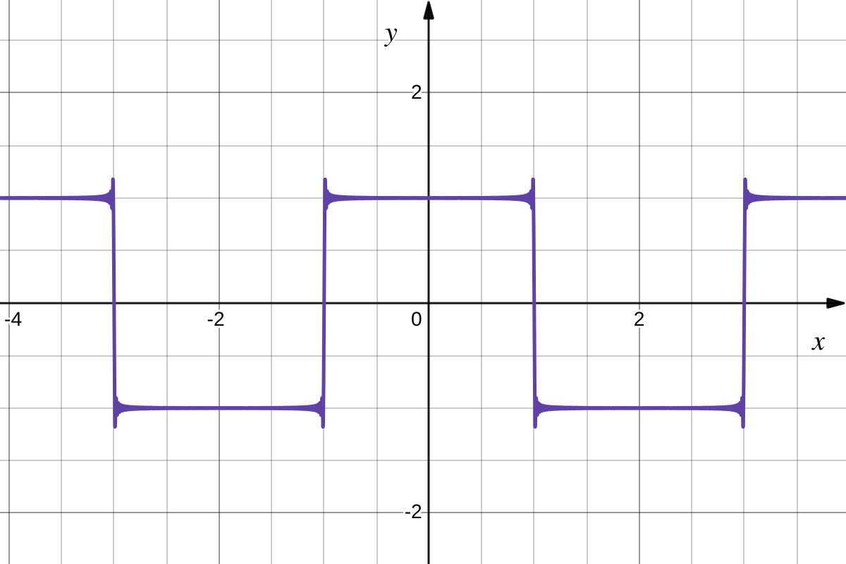
Fig. 2.10 Desmos graph for \(\frac{4}{\pi}\sum_{k=0}^100\frac{(-1)^k}{2k+1}\cos\left(\frac{(2k+1)\pi x}{2}\right)\) (Problem 65).#
This graph was created with \(N=100\), but any \(N>50\) looks similar.
The graph suggests that the infinite series \(\frac{4}{\pi}\sum_{k=0}^\infty\frac{(-1)^k}{2k+1}\cos\left(\frac{(2k+1)\pi x}{2}\right)\) is the Fourier series of the following square wave (see Fig. 2.11).
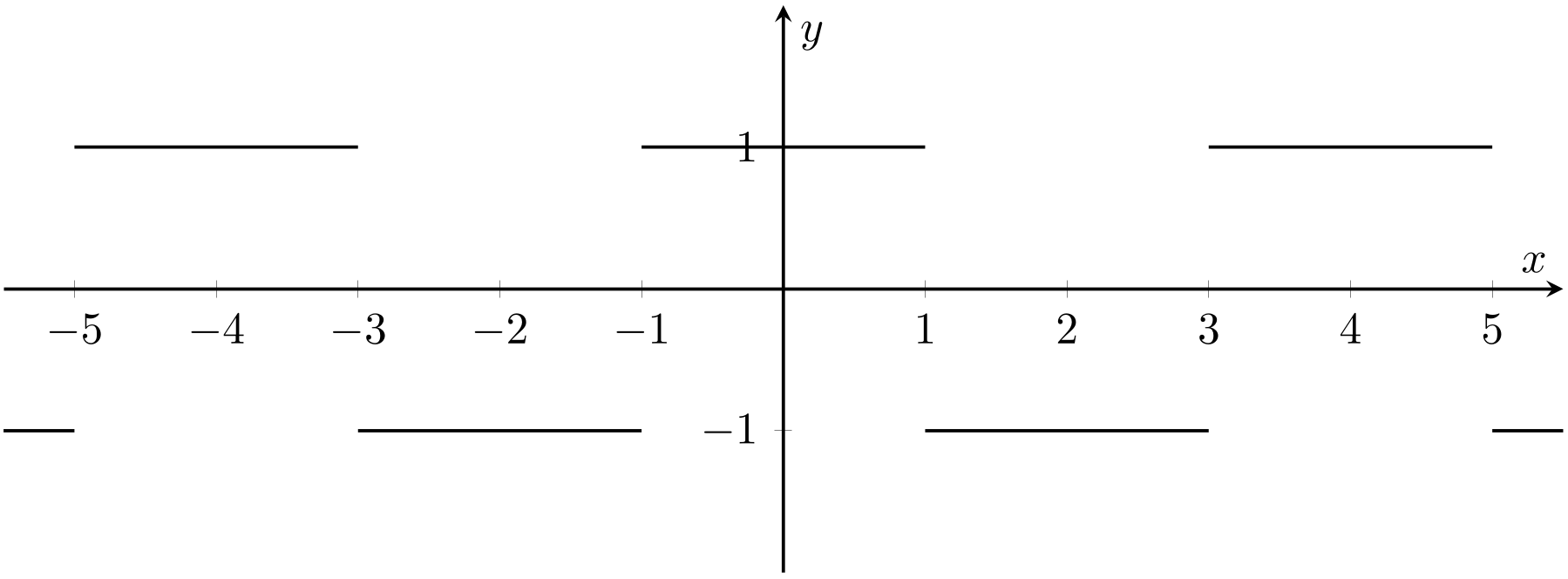
Fig. 2.11 Square wave \(f(x)=\frac{4}{\pi}\sum_{k=0}^\infty\frac{(-1)^k}{2k+1}\cos\left(\frac{(2k+1)\pi x}{2}\right)\) (Problem 65).#
In Fig. 2.11, we have been deliberately vague about the value of \(f(x)\) when \(x\) is an odd integer. In fact, direct calculation using the series shows that \(f(x)=0\) for all odd integer values of \(x\).
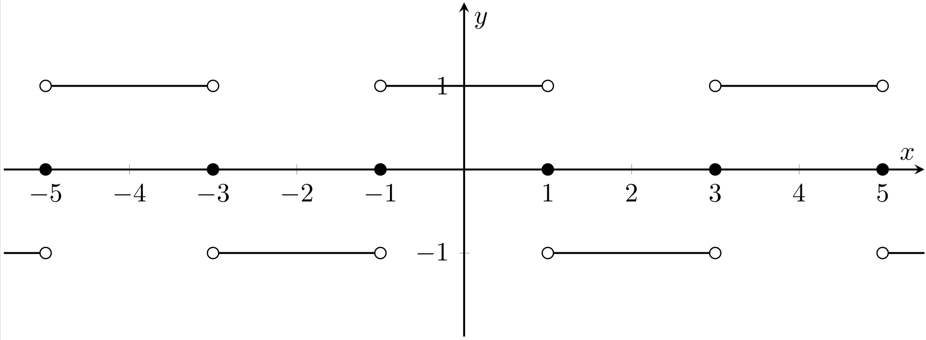
Fig. 2.12 Improved graph of the square wave \(f(x)=\frac{4}{\pi}\sum_{k=0}^\infty\frac{(-1)^k}{2k+1}\cos\left(\frac{(2k+1)\pi x}{2}\right)\) (Problem 65).#
In particular,
Of course, \(f\) is a periodic function with period \(2\).
(ii) We already showed directly in (i) that \(f(x)=0\) whenever \(x\) is an odd integer, but this might not have been obvious from the Desmos graph alone.
(iii) \(f\) is differentiable at all points in \(\mathbb{R}\) except for the odd integers. So \(\text{Dom}(f') = \mathbb{R}\setminus\{2k+1:k\in\mathbb{Z}\}\). For \(x\in\text{Dom}(f')\), \(f'(x)=0\).
(iv) Differentiating the formal series
term-by-term yields
When \(x\) is an even integer, this series converges and equals \(0\). A quick plug into Desmos suggests the series diverges for all other values of \(x\).
Extension: Can you prove this?
Historical note
In Problem 65, we found that at all points aside from the odd integers, the function
is differentiable with derivative equal to \(0\). However, differentiating term-by-term yields a series that diverges for all values of \(x\) except the even integers.
It was apparent contradictions such as this that created such a stir among the contemporaries of Fourier, and meant his 1807 paper was never accepted for publication. As modern mathematicians, we have access to subtle ideas like uniform and absolute convergence (not to mention a functioning definition of differentiability) that allow us to make sense of the strange behaviour exhibited by this series. Mathematicians of the early 19th century could not reconcile the obvious usefulness of the method Fourier had showcased with everything they knew or believed to be true about functions, series and derivatives.
Following these events was a huge collective effort of the whole mathematical community to properly understand and develop rigorous foundations for calculus — or as it came to be known, real analysis.
Disclaimer: I am not a historian. For more on this fascinating subject, I recommend reading Chapter 1 of A Radical Approach to Real Analysis by Bressoud.
2.6. Integration — Non-examinable 2024–25#
66. Let \(f:[1,4]\to\mathbb{R}\); \(f(x)=\frac{1}{x}\), and let \(P=\{1,\frac{3}{2},2,4\}\).
(i) Below (Fig. 2.13) is a sketch of the graph of \(f\), the partition \(P\), and the associated upper and lower Riemann sums.
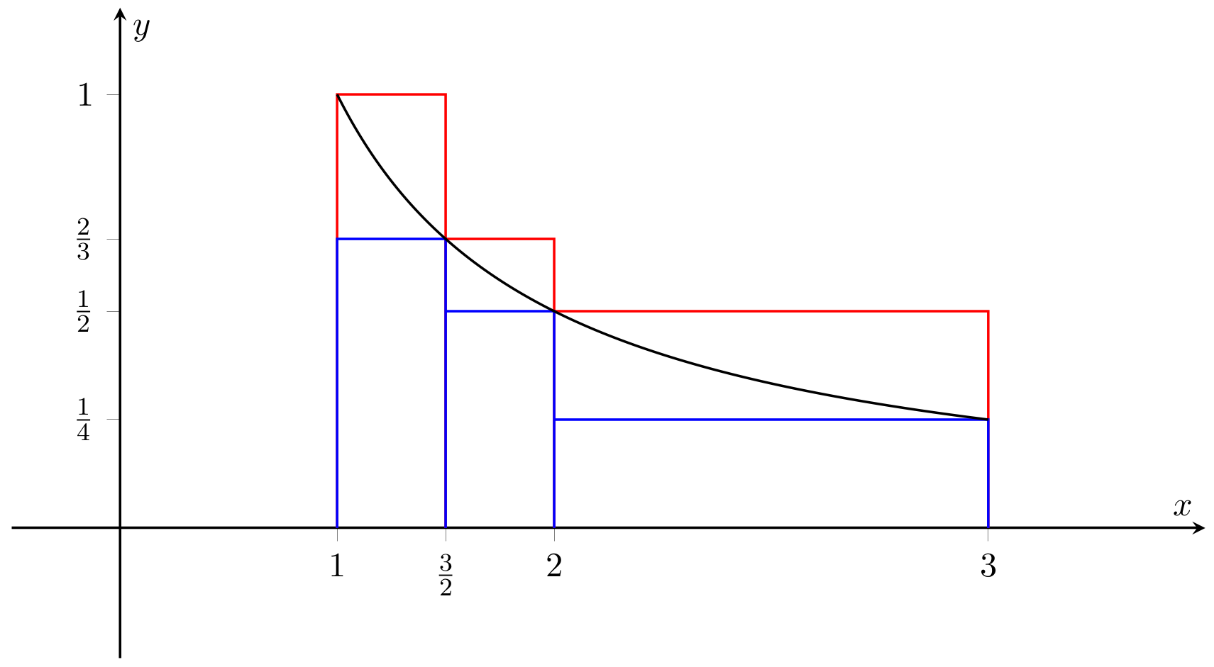
Fig. 2.13 \(y=\frac{1}{x}\), with upper and lower sums (Problem 66(i)).#
We have \(U(f,P) = \sum_{k=1}^4M_k(x_k-x_{k-1})\), where \(x_0=1\), \(x_1=\frac{3}{2}\), \(x_2=2\), \(x_3=4\), and
Therefore,
Similarly, \(L(f,P) = \sum_{k=1}^4m_k(x_k-x_{k-1})\), where
and
Hence
and so
(ii) Adding the point \(P\) has the following effect (Fig. 2.14)
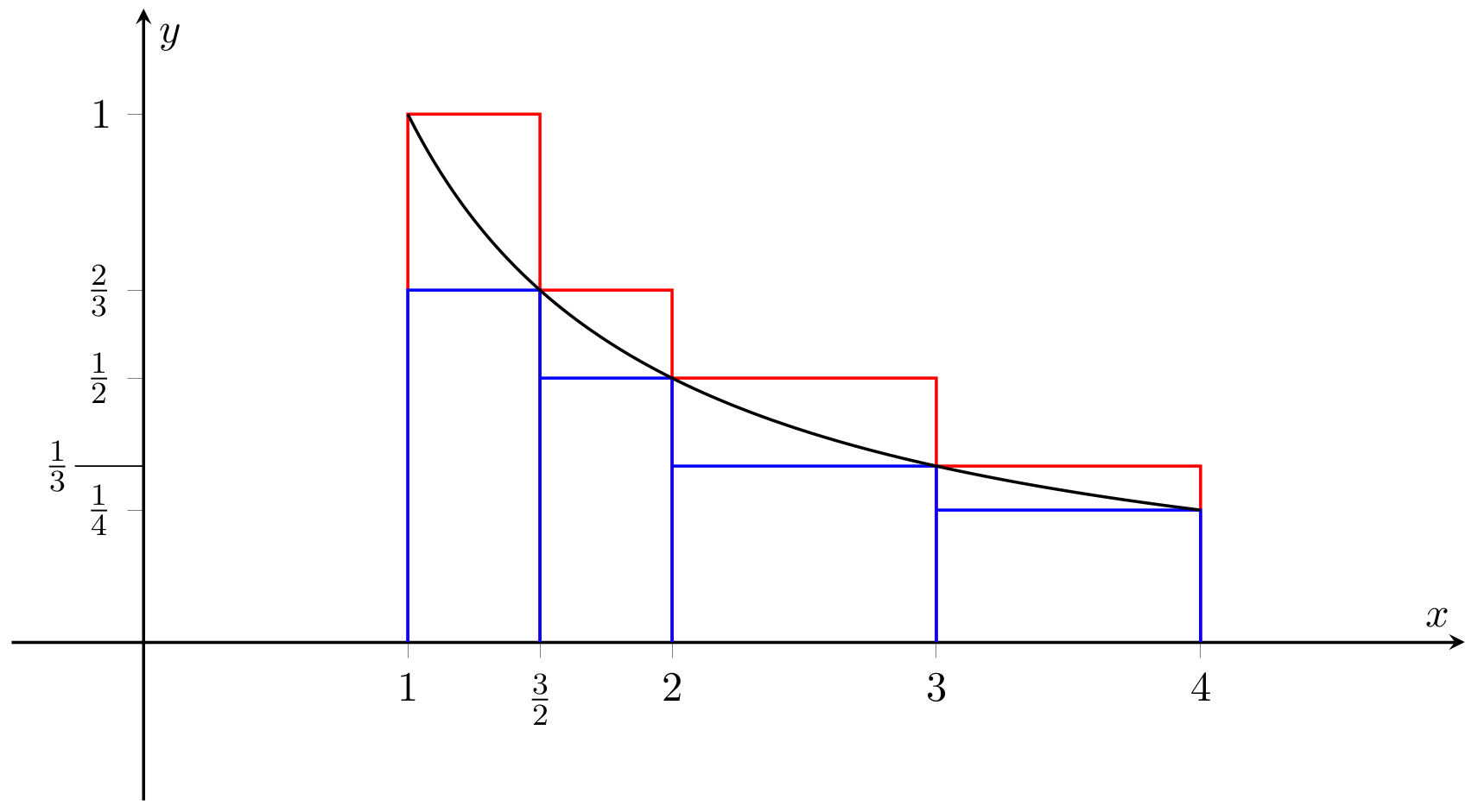
Fig. 2.14 Upper and lower sums with additional point \(3\) (Problem 66(ii)).#
We now have \(x_0=1\), \(x_1=\frac{3}{2}\), \(x_2=2\), \(x_3=3\) and \(x_4=4\). \(M_1\), \(M_2\), \(m_1\) and \(m_2\) are not affected by the additional point, while
Therefore
and
So the size of \(U(f,P)-L(f,P)\) has decreased after adding the point \(3\) to \(P\).
(iii) Mimicking the proof of Theorem 6.1, let \(x_k=1+\frac{3}{n}k\) for \(k=0,\ldots,n\). Then, \(P=\{x_0,\ldots,x_n\}\) partitions \([1,3]\) uniformly into \(n\) intervals, each of width \(\frac{3}{n}\). Since \(\frac{1}{x}\) is decreasing,
and
for each \(k\). So,
We have been asked to find \(P\) so that \(U(f,P)-L(f,P)<\frac{2}{5}\), so we choose \(n\) so that \(\frac{9}{4n}<\frac{2}{5}\). That is, \(n>\frac{45}{8}\). In fact, \(n=6\) will do.
So \(x_k=1+\frac{1}{2}k\) for \(k=0,\ldots,6\), and \(P=\left\{1,\frac{3}{2},2,\frac{5}{2},3,\frac{7}{2},4\right\}\).
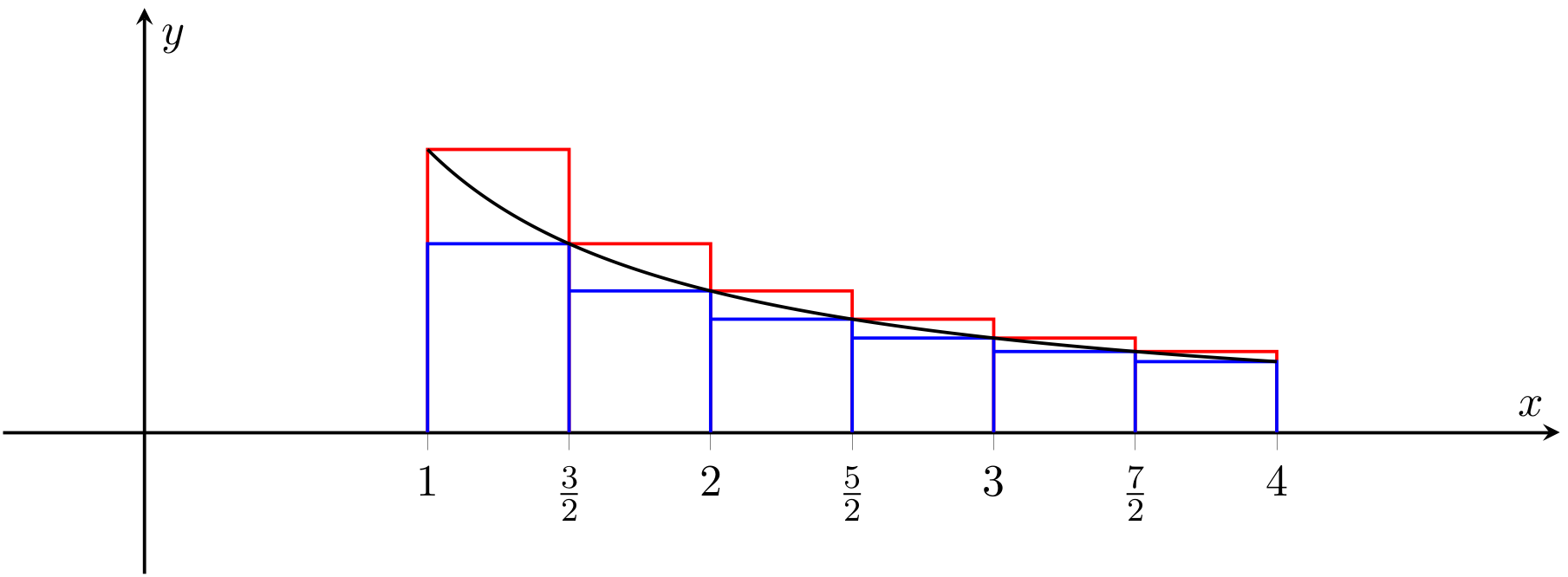
Fig. 2.15 Q66: A partition for which \(U(f,P)-L(f,P)<\frac{2}{5}\) (Problem 66(iii)).#
67. Let \(g:[0,1]\to\mathbb{R}\); \(\displaystyle g(x)=\left\{\begin{array}{cc} 1 & \text{for } 0\leq x<1 \\ 2 &\text{for } x=1 \end{array}\right.\).
(i) Let \(P=\{x_0,x_1,\ldots x_n\}\) be any partition \([0,1]\), with \(0=x_0<x_1<\ldots<x_n=1\). Then for \(k=1,\ldots n\),
Therefore
(ii) Since \(g\) is constant on \([0,1)\), we may as well take a partition consisting of 3 points — the end points and a single point in the middle.
Let \(\delta>0\) and consider the partition \(P=\{0,1-\delta,1\}\) of \([0,1]\) (see Fig. 2.16).
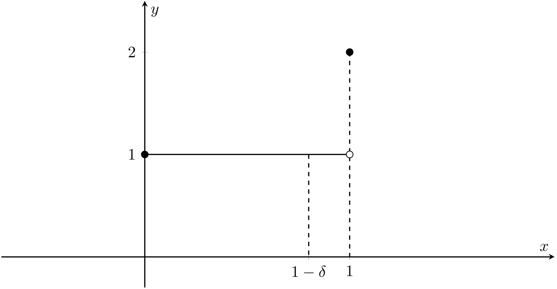
Fig. 2.16 Graph of \(g\) with partition \(P=\{0,1-\delta,1\}\) (Problem 67).#
Making \(\delta\) smaller should reduce the size of \(U(g,P)\). We have
so
Taking \(\delta=\frac{1}{10}\) will give \(U(g,P)=1+\frac{1}{10}\). So our choice of partition should be \(P=\left\{0,\frac{9}{10},1\right\}\).
(iii) By (ii), taking \(P=\left\{0,1-\frac{\varepsilon}{2},1\right\}\) will give \(U(g,P)=1+\frac{\varepsilon}{2} < 1+\varepsilon\).
By (i), \(L(g,P)=1\), and so we’ve found a partition \(P\) so that \(U(g,P)-L(g,P)<\varepsilon\). This proves \(g\) is Riemann integrable (by Proposition 6.1).
68. For \(\mathbb{1}_{[a,b]}\), this is just a special case of Example 6.2, and there is nothing to show.
Note also that for any partition \(P\) of \([a,b]\),
This is because each of these functions have supremum \(1\) on any subinterval of \([a,b]\).
For the lower integrals, let’s first consider \(\mathbb{1}_{(a,b]}\). Consider the partition \(P=\{a,a+\delta,b\}\) (see Fig. 2.17).

Fig. 2.17 Graph of \(\mathbb{1}_{(a,b]}\), with partition \(P=\{a,a+\delta,b\}\) (Problem 68).#
Then \(U(\mathbb{1}_{(a,b]},P) = b-a\) as before, while
Therefore, \(U(\mathbb{1}_{(a,b]},P) -L(\mathbb{1}_{(a,b]},P) = \delta\) for this partition \(P\).
We can now use Proposition 6.1: given \(\varepsilon>0\), the partition \(P_\varepsilon:=\left\{a,a+\frac{\varepsilon}{2},b\right\}\) gives
and so \(\mathbb{1}_{(a,b]}\) is Riemann integrable.
To evaluate \(\int_a^b\mathbb{1}_{(a,b]}(x)dx\), note that by our work above,
Since this is true for all \(\varepsilon\), the only option is for \( \int_a^b\mathbb{1}_{(a,b])}(x)dx = b-a\).
The proof that \(\mathbb{1}_{[a,b)}\) is integrable with \(\int_a^b\mathbb{1}_{[a,b)}(x)dx = b-a\) is nearly identical — just consider the partitions of the form \(P=\{a,b-\delta,b\}\) instead.
For \(\mathbb{1}_{(a,b)}\), let \(\delta>0\), and consider \(P=\{a,a+\delta,b-\delta,b\}\). As before, \(U(\mathbb{1}_{(a,b)},P)=b-a\), and direct calculation gives
Then, given \(\varepsilon>0\), take \(\delta=\frac{\varepsilon}{4}\). We get
and so \(\mathbb{1}_{(a,b)}\) is integrable, by Proposition 6.1. Moreover,
and since this is true for all \(\varepsilon>0\), we must have \(\int_a^b\mathbb{1}_{(a,b)}(x)dx =b-a\).
69. (i) By results from the course (specifically, Propositions 6.2 and Proposition 6.3(ii)), \(r\) and \(s\) are both linear combinations of integrable functions, and hence are integrable with
and
(ii) Continuous functions are integrable, by another result from the course (specifically, by Theorem 6.2). So \(f\colon [0,3]\rightarrow \mathbb{R}\) defined by \(f(x)=e^{x^2}\) is integrable since it is a continuous function.
[Alternative answer: by the fact \(f\) is monotonic increasing (c.f. Theorem 6.1).]
(iii) Note that \(r(t)\leq f(t)\leq s(t)\) for all \(t\), and so by Proposition 6.3(i),
70. Let \(f,g:[a,b]\to\mathbb{R}\) be integrable functions.
(i) For any subset \(A\subset[a,b]\),
and similarly
It is then immediate from the definition of the upper and lower sums that
and
For the example where this is strict, a good strategy is to look for functions with features that “cancel out” in some sense. For example, you could take
and
Then \(f+g\) is the zero function, so \(L(f+g,P)=U(f+g,P)=0\). On the other hand
and
(ii) Let \(P_1\) and \(P_2\) be partitions of \([a,b]\). Then
by Lemma 6.1, since \(P_1\cup P_2\) is a refinement of both partitions \(P_1\) and \(P_2\).
The proof of the lower sum statement is similar:
(iii) We just proved
for all partitions \(P_1\) and \(P_2\) of \([a,b]\).
Taking \(\inf\) over \(P_1\),
and then taking \(\inf\) over \(P_2\),
Since \(f\) and \(g\) are integrable, \(\int_a^bf(x)dx=U(f)\) and \(\int_a^bg(x)dx=U(g)\). This shows that
A similar argument shows that
Hence
The only option is
That is, \(f+g\) is integrable and
71. Let \(P\) be the partition \(a=x_0<x_1<\ldots<x_n=b\). If \(k\geq 0\), then
and
Therefore \(U(kf,P)=kU(f,P)\) and \(L(kf,P)=kL(f,P)\), and taking infima/suprema, \(U(kf)=kU(f)\) and \(L(kf)=kL(f)\).
Since \(f\) is integrable, \(U(f)=L(f)=\int_a^bf(x)dx\), and hence
It follows that \(kf\) is integrable, with \(\displaystyle\int_a^bkf(x)dx=k\int_a^bf(x)dx\).
To extend this result to include negative \(k\), it is sufficient to prove the \(k=-1\) case. Note that
and
Therefore, \(U(-f,P)=-L(f,P)\) and \(L(-f,P)=-U(f,P)\), and so
Similarly,
Therefore \(U(-f) = -L(f) = -U(f) = L(-f)\), so \(-f\) is integrable, and
72. We have: \(M=\sup\{f(x):x\in A\}, \; m=\inf\{f(x):x\in A\}\), and \(M'=\sup\{|f(x)|:x\in A\}, \; \text{ and } \; m'=\inf\{|f(x)|:x\in A\}\).
(i) Case 1: \(m\geq 0\). Then \(f\) is a non-negative function, so \(M=M'\), \(m=m'\), and \(M-m=M'-m'\).
Case 2: \(m\leq M\leq 0\). Then \(M'=-m\), \(m'=-M\), and so again \(M'-m'=M-m\).
Case 3: \(m<0<M\). Then \(M'=\max\{M,-m\}\leq M+(-m)\), since both \(M\) and \(-m\) are positive numbers. Then,
since \(m'\geq 0\).
(ii) Let \(f:[a,b]\to\mathbb{R}\) be integrable, and let \(P\) be the partition \(a=x_0<x_1<\ldots<x_n=b\). For \(k=1,\ldots,n\). let
Then by part (i), \(M_k-m_k\geq M_k'-m_k'\) for each \(k\). Therefore,
(iii) Since \(f\) is integrable, for all \(\varepsilon>0\), we can choose the a partition \(P\) so that \(U(f,P)-L(f,P)<\varepsilon\). Using the result of part (ii). it follows that \(U(|f|,P)-L(|f|,P)<\varepsilon\) for this partition, and so \(|f|\) is integrable.
Since \(-|f(x)|\leq f(x)\leq |f(x)|\) for all \(x\in[a,b]\), Proposition 6.3(iii) implies that
That is,
73. We have
Write \(F:\mathbb{R}\to\mathbb{R}\); \(F(x)=\int_0^x f(t)dt.\) Then by the fundamental theorem of calculus (Theorem 6.3), \(F\) is differentiable, and \( F'(x)=f(x)\) for all \(x\in\mathbb{R}\). Also,
and \(b\) is differentiable. Therefore, by the chain rule (Theorem 4.4), \(F\circ b\) is also differentiable, with
for all \(x\in\mathbb{R}\). Similarly,
Subtracting these
as required.
74. (i) It follows immediately from the fundamental theorem of calculus that \(l\) is differentiable, with \(l'(x)=\frac{1}{x}\).
(ii) By Proposition 6.3 in the lecture notes,
In the second integral, set \(a(x)=xy\), \(b(x)=x\) and use Problem 72. We have \(a'(x)=y\) and \(b'(x)=1\), so
Therefore \(\int_x^{xy}\frac{1}{t}dt\) is constant as a function of \(x\). In particular, it coincides with its value when \(x=1\):
and \(l(xy)=l(x)+l(y)\) follows.
75.* Define \(G\colon [a,b]\rightarrow \mathbb{R}\) by
Then \(G\) is a continuous function. This was mentioned in the lectures. To see why, let \(h>0\). Since the function \(f\) is Riemann integrable, it is bounded, so we have \(M\in \mathbb{R}\) such that \(|f(t)|\leq M\) for all \(t\in [a,b]\). Then
Similarly \(|G(x-h) - G(x) | \leq Mh\).
So \(G(x+h)\rightarrow G(x)\) as \(h\rightarrow 0\), and \(G\) is continuous.
Thus we can define a continuous function \(F\colon [a,b]\rightarrow \mathbb{R}\) by
Observe that
If \(\int_a^b f(t)\, dt =0\), then we can take \(x=a\) and we have the required result. Otherwise, either \(F(a)<0\) and \(F(b)>0\) or \(F(a)>0\) and \(F(b)<0\).
Either way, by the intermediate value theorem, we have \(x\in [a,b]\) such that \(F(x)=0\), that is to say
76. (i) Let \(\mu = \frac{1}{b-a} \int_a^b f(x)\, dx\). Then \(\int_a^b f(x)\, dx=(b-a)\mu\), and we need only show that \(\mu\in[m,M]\).
Consider the step functions \(m\mathbf{1}_{[a,b]}\) and \(M\mathbf{1}_{[a,b]}\) with \(m\mathbf{1}_{[a,b]}(x)\leq f(x)\leq M\mathbf{1}_{[a,b]}(x)\) for all \(x\in[a,b]\). Thus we have
But \(\int_a^b f(x)\, dx=(b-a)\mu\), and so \(\mu \in [m,M]\).
(ii) We are now given that \(f:[a,b]\to\mathbb{R}\) is continuous. By Corollary 3.3, \(f([a,b])=[m,M]\), where
In particular, \(m<f(x)<M\) for all \(x\in[a,b]\), and so by part (i),
for some \(\mu \in [m,M]\). As \(\mu\in [m,M]=f([a,b])\) and \(f\) is continuous, there is some \(\xi \in [a,b]\) such that \(f(\xi ) = \mu\). Hence
77. Let \(f:[a,b]\to\mathbb{R}\) be continuous, and \(m = \inf \{ f(x) : x\in [a,b] \}\) and \(M = \sup \{ f(x) : x\in [a,b] \}\) as before. Then \(m\leq f(x)\leq M\) for all \(x\in [a,b]\). As \(g(x)\geq 0\), we have
for all \(x\in [a,b]\). By Proposition 6.3(i),
Let
Either \(I=0\) or \(I>0\). If \(I=0\), then the above tells us that
and any \(\xi \in [a,b]\) satisfies
If \(I>0\), then
By Corollary 3.3, \(f([a,b])=[m,M]\), and so there is \(\xi \in [m,M]\) such that
or in other words
We do need the assumption \(g(x)\geq 0\). To see this, consider the function \(g(x) = x\) for \(x\in [-1,1]\). Then
so the result would say that for any continuous function \(f\colon [-1,1]\rightarrow \mathbb{R}\) we have
But this is clearly not the case, taking for example \(f(x)=x\).