Continuity

3. Continuity#

3.1. Definition of continuity, basic properties and examples#

Intuitively we think of functions as being “continuous” if we can draw their graphs without ever taking our pen/pencil off the paper: the graph contains no gaps/jumps/discontinuities. So if we think of a typical point $a$ in the domain of the function $f$, then as $x$ gets closer and closer to $a$, we expect that $f(x)$ will get closer and closer to $f(a)$. But from the work of Chapter 2, recall that as $x$ gets closer and closer to $a$, then $f(x)$ gets closer and closer to its limit at $a$ (if this exists). This leads to the following definition.

Definition 3.1 (Continuity)

Let $f:X\to\mathbb{R}$ where $X$ is a subset of $\mathbb{R}$ and let $a\in X$.

We say that $f$ is continuous at the point $a$ if $\lim_{x \rightarrow a}f(x)$ exists and equals $f(a)$.

We say that $f$ is continuous on a set $S \subseteq X$ if it is continuous at every point of $S$.

Example 3.1

Let $f:\mathbb{R}\to\mathbb{R}$, $f(x)=3+x-x^2$. Let’s show this function is continuous at $x=2$. This means proving that $f(x)\rightarrow f(2)$ as $x\rightarrow 2$.

Let $\varepsilon>0$. We seek $\delta>0$ such that $|f(x)-f(2)|<\varepsilon$ whenever $0<|x-2|<\delta$. Now, for all $x\in\mathbb{R}$,

\[\begin{align*} |f(x)-f(2)| &= |3+x-x^2 - (3+2-2^2)| \\ &= |x-x^2+2| \\ &= |x^2-x-2| \\ &= |x+1||x-2|. \end{align*}\]

Let’s bound $|x+1|$ first. Note that if $|x-2|<1$, then $1<x<3$, so $2<x+1<4$. Therefore, $|x-2|<1$ implies

\[ |f(x)-f(2)| = |x+1||x-2|< 4|x-2|. \]

We can make this less than $\varepsilon$ by taking $\delta:=\min\left\{1,\frac{\varepsilon}{4}\right\}$.

Indeed, for this $\delta$, $0<|x-2|<\delta$ implies that both inequalities $0<|x-2|<1$ and $0<|x-2|<\frac{\varepsilon}{4}$ hold simultaneously. Thus,

\[ |f(x)-f(2)| = |x+1||x-2| < 4|x-2| < 4\cdot\frac{\varepsilon}{4} =\varepsilon. \]

Hence $\lim_{x\rightarrow 2}f(x)=f(2)$, and $f$ is continuous at $2$.$\square$

Just as we had a sequential criterion for limits of functions, there is an equivalent, sequential definition for continuity of functions. We summarise the various equivalent definitions below.

Theorem 3.1 (Sequential criterion for continuity)

Let $f:X\to\mathbb{R}$ where $X$ is a subset of $\mathbb{R}$ and let $a\in X$ be a limit point of $X$.

Then the following statements are equivalent.

(i) $f$ is continuous at $a$.

(ii) Given any sequence $(x_{n})$ with $x_{n} \in X$ for all $n\in\mathbb{N}$, such that $\lim_{n \rightarrow \infty}x_{n} = a$, we have $\lim_{n\rightarrow\infty} f(x_{n}) = f(a)$.

(iii) Given any $\varepsilon > 0$, there exists $\delta > 0$ such that whenever $x \in X$ with $|x - a| < \delta$, we have $|f(x) - f(a)| < \varepsilon$.

Proof. The proof that (ii) and (iii) are equivalent is almost exactly the same as the proof of Theorem 2.1.

We prove that (i) and (iii) are equivalent. By Definition 3.1, (i) is equivalent to: $\lim_{x \rightarrow a}f(x)$ exists and equals $f(a)$.

By Definition 2.2, this is equivalent to

(iii)’: For all $\varepsilon>0$ there exists $\delta>0$ such that for all $x\in X$, $0<|x-a|<\delta$ implies $|f(x)-f(a)|<\epsilon$.

Let’s check that (iii) and (iii)’ are equivalent. The only difference is whether or not we allow $x=a$. But in the case where $x=a$, we get $|f(x)-f(a)|=0<\varepsilon$, and so there is nothing more to show. $\square$

Remark 3.1

We can rewrite Theorem 3.1(iii) as

“Given any $\varepsilon > 0$, there exists $\delta > 0$ such that whenever $x \in X$ with $x \in (a -\delta, a + \delta)$, we have $f(x) \in(f(a) - \varepsilon, f(a) + \varepsilon)$.”

An open interval of the form $(a - \delta, a + \delta)$, where $\delta > 0$ is called an open neighbourhood of $a \in \mathbb{R}$. This reformulation of the notion of continuity in terms of open neighbourhoods is better suited in more advanced topics, such as analysis with functions on $\mathbb{R}^n$, or more generally still, functions on a metric or topological space[1].

Just as with functional limits, the sequential criterion for continuity is often much easier to employ in proofs.

Example 3.2 (Constant functions)

Fix $c \in \mathbb{R}$, then the constant function $f:\mathbb{R}\to\mathbb{R}$ given by $f(x) = c$ is continuous on $\mathbb{R}$. To see this, let $a \in \mathbb{R}$ be arbitrary and let $(x_{n})$ be any sequence converging to $a$. Then $f(x_{n}) = c$ for all $n\in\mathbb{N}$ and so the sequence $(f(x_{n}))$ clearly converges to $c = f(a)$. Thus the function is continuous at $a$.

Example 3.3 (Identity function)

The linear function $f:\mathbb{R}\to\mathbb{R}$ given by $f(x) = x$ is also continuous on $\mathbb{R}$. Again given any sequence $(x_{n})$ converging to $a$, $f(x_{n}) = x_{n}$ for all $n\in\mathbb{N}$, and so the sequence $(f(x_{n}))$ clearly converges to $f(a) = a$.

To build more interesting examples, we need the following.

Theorem 3.2 (Algebra of continuous functions)

Suppose that $f:A\to\mathbb{R}$ and $g :B \rightarrow \mathbb{R}$ are both continuous at $a \in A\cap B$. The following functions are also continuous at $a$.

(i) $f + g$,

(ii) $fg$,

(iii) $\alpha f$, for all $\alpha \in \mathbb{R}$,

(iv) $\displaystyle\frac{f}{g}$, provided $g(a) \neq 0$.

Proof. This is a direct consequence of Theorem 2.2. $\square$

Remark 3.2 (Vector spaces of continuous functions)

In Semester 1, those taking MAS2004 worked with $C(X)$, the set of all continuous functions with domain $X$, where $X\subseteq\mathbb{R}$. Theorem 3.2 takes care of the “hard” part of proving this set is a vector space — that is, showing it is closed under addition and scalar multiplication.

Using algebra of limits and Example 3.2 and Example 3.3, we can expand our supply of continuous functions.

Example 3.4 (Polynomial functions)

Using Theorem 3.2(ii) and induction, show that $f(x) = x^{k}$ is continuous on $\mathbb{R}$, for all $k\in\mathbb{N}\cup\{0\}$.

Prove that polynomial functions

\[ p(x) = a_{0} + a_{1}x + \cdots + a_{n}x^{n} \]

are continuous on the whole of $\mathbb{R}$.

Example 3.5 (Rational functions)

Using Example 3.4 and Theorem 3.2(iv), we can also conclude that rational functions $r(x) = \frac{p(x)}{q(x)}$ are continuous at every point where $q(x)\neq 0$.

The continuity on $\mathbb{R}$ of functions such as $f(x) = e^{k x}, g(x) = \sin(kx), h(x) = \cos(kx)$, for $k \in \mathbb{R}$, can be established using power series arguments. We will explore this further in Chapter 5.

We also have a result for composition of functions.

Definition 3.2 (Composition of functions)

Recall that the composition $g \circ f$ of two functions $f:X\to Y$ and $g:Y\to Z$ is defined to be the function $g\circ f: X\to Z$, given by

\[ (g \circ f)(x) = g(f(x)). \]

Of course, the order of composition matters: we typically do not have $f \circ g = g \circ f$, even at points where both are defined. For example, if $f:\mathbb{R}\to\mathbb{R}$ is given by $f(x)=x+2$ and $g:\mathbb{R}\to\mathbb{R}$ is given by $g(x)=3x$ then $g\circ f:\mathbb{R}\to\mathbb{R}$ given by $(g\circ f)(x)=3x+6$, whereas $f\circ g:\mathbb{R}\to\mathbb{R}$ given by $(f\circ g)(x)=3x+2$.

Theorem 3.3 (Composition of continuous functions)

Let $f:A\to B$ and $g:B\to \mathbb{R}$, so we have the composition $g\circ f: A\to \mathbb{R}$, given by $ (g \circ f)(x) = g(f(x))$. If $f$ is continuous at $a$ and $g$ is continuous at $f(a)$, then $g \circ f$ is continuous at $a$.

Proof. This is for you to do in Problem 15. $\square$

With Theorem 3.3, we can immediately deduce continuity for an even wider range of functions.

Example 3.6

Let $f:\mathbb{R}\to\mathbb{R}$; $f(x)=\sqrt{x^2+1}$. Then $f=g\circ h$, where $g:[0,\infty)\to\mathbb{R}$; $g(x)=\sqrt{x}$, and $h:\mathbb{R}\to\mathbb{R}$, $h(x)=x^2+1$. A quick check shows this is well-defined: if $x\in\mathbb{R}$, then $h(x)\in[0,\infty)$, so $g\circ h(x)=g(h(x))$ makes sense.

Both $g$ and $h$ are continuous on their domains: for $g$, this follows from Problem P4(iii), and for $h$, it is immediate from our observations about polynomials (c.f. Example 3.4).

Therefore, by theorem Theorem 3.3, $f$ is continuous on all of $\mathbb{R}$.

Remark 3.3 (Trig and exponential functions)

Our work in Chapter 5 will enable us to formally define trigonometric and exponential functions via their power series, and prove they are continuous. For now, we assume these functions are continuous without proof, as it allows us to consider some interesting examples.

Continuous extensions

Definition 3.3 (Continuous extensions)

Given two functions $f_{1}:A\to\mathbb{R}$ and $f_{2}:B\to \mathbb{R}$, we say that $f_{2}$ is an extension of $f_{1}$, (and that $f_{1}$ is a restriction of $f_{2}$) if $A \subseteq B$ and $f_{1}(x) = f_{2}(x)$ for all $x \in A$. If $f_{1}$ is continuous on $A$ and $f_{2}$ is continuous on $B$, we say that $f_{2}$ is a continuous extension of $f_{1}$ (to $B$).

Example 3.7

Consider the function $g: \mathbb{R} \setminus \{0\}\to\mathbb{R}$ given by

\[ g(x) = x\sin\left(\frac{1}{x}\right). \]

Subject to the assumption that $\sin$ is continuous on $\mathbb{R}$, we can deduce ussing Theorem 3.2 and Theorem 3.3 that $g$ is continuous at every point of its domain. In Problem 10, you showed that $\displaystyle\lim_{x \rightarrow 0}g(x)$ exists and is $0$.

Now, we may define a new function $\tilde{g}:\mathbb{R}\to\mathbb{R}$ by

\[\begin{split} \tilde{g}(x) = \begin{cases} g(x) &\text{if $x \in \mathbb{R} \setminus \{0\}$},\\ 0&\text{if $x= 0$}. \end{cases} \end{split}\]

Then $\tilde{g}$ is a continuous extension of $g$ to the whole of $\mathbb{R}$.

On the other hand, consider the function

\[ h: \mathbb{R} \setminus \{0\}\to\mathbb{R}; \hspace{1em} h(x) = \sin\left(\frac{1}{x}\right). \]

This function has many extensions to the whole of $\mathbb{R}$: we could, for example, define

\[\begin{split} \tilde{h}(x) = \left\{\begin{array}{l c} h(x) & ~\mbox{if}~x \neq 0\\ 0& ~\mbox{if}~x = 0 \end{array} \right., \end{split}\]

but since, as was shown in Problem 9, $\displaystyle\lim_{x \rightarrow 0}h(x)$ does not exist, there are no continuous extensions of $h$ to $\mathbb{R}$.

3.2. Discontinuity#

Definition 3.4 (Discontinuity)

A function $f:X \rightarrow \mathbb{R}$ is said to have a discontinuity at $a \in X$ if it fails to be continuous there. In this case we say that $f$ is discontinuous at $a$.

3.2.1. Left- and right-continuity; jump discontinuities#

Discontinuities can be very strange. However, like with divergence, there are some caregories of “nice” discontinuity, and we discuss this next.

Example 3.8

Consider the Heaviside function, $\mathbb{1}_{[0,1]}$ (known as the Heaviside function). Common sense tells us that $\mathbb{1}_{[0,1]}$ has discontinuities at $0$ and $1$, and is continuous everywhere else in its domain.

Let’s prove discontinuity at $0$ rigorously. If $\mathbb{1}_{[0,1]}$ were continuous at $0$, then Theorem 3.1 would imply that for any sequence $(x_n)$ converging to $0$, the sequence $\mathbb{1}_{[0,1]}(x_n)$ should converge to $\mathbb{1}_{[0,1]}(0) = 1$.

Consider the sequence $(x_n)$ given by $x_n=-\frac{1}{n}$, for each $n\in\mathbb{N}$. Certainly $\lim_{n\rightarrow\infty}x_n=0$. Also, since $x_n<0$ for all $n\in\mathbb{N}$, we have $\mathbb{1}_{[0,1]}(x_n) = 0$ for all $n\in\mathbb{N}$. Therefore,

\[ \lim_{n\rightarrow\infty}\mathbb{1}_{[0,1]}(x_n) = \lim_{n\rightarrow\infty} 0 = 0 \neq \mathbb{1}_{[0,1]}(0). \]

We have arrived at a contradiction, and so $\mathbb{1}_{[0,1]}$ has a discontinuity at $0$.

More generally, the indicator function $\mathbb{1}_{[a, b]}:\mathbb{R}\to\mathbb{R}$ is discontinuous at $a$, and at $b$, but is continuous on $\mathbb{R} \setminus \{a, b\}$. To show that a function is discontinuous at $a$, it is sufficient to find a single sequence $(x_{n})$ in $X \setminus \{a\}$, such that $\lim_{n \rightarrow \infty}x_{n} = a$, but $\lim_{n \rightarrow \infty}f(x_{n}) \neq f(a)$.

We can learn more about what happens at a discontinuity by using right and left limits.

Definition 3.5 (Left and right continuity)

We say that $f:X\to\mathbb{R}$ is left continuous at $a \in X$ if $\lim_{x \rightarrow a^-}f(x) = f(a)$, and right continuous at $a \in X$ if $\lim_{x \rightarrow a^+}f(x) = f(a)$.

Example 3.9

The function $\mathbb{1}_{[a, b]}:\mathbb{R}\to\mathbb{R}$ is left continuous at $x = b$, and right continuous at $x = a$.

Solution. We just prove the right continuity, as the other argument is so similar. Let $(x_{n})$ be any sequence with $x_{n} > a$ for all $n\in\mathbb{N}$ that converges to $a$. Then for sufficiently large $n$, $x_n\in(a,b]$ and $\mathbb{1}_{[a, b]}(x_{n}) = 1$, so $\lim_{n\rightarrow\infty} \mathbb{1}_{[a, b]}(x_{n}) = 1 = \mathbb{1}_{[a, b]}(a)$, and the result follows.

Exercise. Prove that a function $f: X \rightarrow \mathbb{R}$ is continuous at $a \in X$ if and only if it is both right and left continuous there.

Definition 3.6 (Jump discontinuity)

If $f$ is discontinuous at $a$ but both $\lim_{x \rightarrow a^-}f(x)$ and $\lim_{x \rightarrow a^+}f(x)$ exist (i.e. they are real numbers) and are unequal, we say that $f$ has a jump discontinuity at $a$. A typical example of this is a step function, or an indicator function $\mathbb{1}_{[a, b]}$, where $[a,b]\subseteq\mathbb{R}$ is some interval.

3.2.2. Stranger discontinuities#

More generally, there is no reason to expect points discontinuity to behave in as straightforward or quantifiable a way as with jump discontinuities. We discuss two famous examples next that illustrate this. What is hopefully satisfying to note is that we would have no way of analysing these functions had we not put the time in to develop a rigorous notion of limits and continuity. (Mathematicians of the 18th century wouldn’t stand a chance.)

Example 3.10 (Dirichlet’s function)

Show that the function $\mathbb{1}_{\mathbb{Q}}:\mathbb{R}\to\mathbb{R}$ is discontinuous at every point in $\mathbb{R}$.

Solution. For convenience, write $f = \mathbb{1}_{\mathbb{Q}}$. Then $f(x) = 1$ if $x$ is rational, and $0$ if it is irrational.

First we will show that $f$ is discontinuous at any given point $a \in \mathbb{Q}$. For this, we need only find one sequence $(a_n)$ converging to $a$ for which $\lim_{n\rightarrow\infty}f(a_n)\neq f(a)$.

Consider first the sequence with $n^{\text{th}}$ term given by $a+\frac{1}{n}$.

Every term in this sequence is rational, and hence for every $n$ we may choose an irrational $a_n$ for which

\[ a < a_{n} < a+\frac{1}{n}. \]

By the squeeze theorem, $\lim_{n\rightarrow\infty} a_{n} = a$, but $\lim_{n\rightarrow\infty} f(a_{n}) = 0 \neq 1 = f(a)$. Hence $f$ is discontinuous at $a$, for all $a\in\mathbb{Q}$.

Now suppose that $a$ is irrational. Since the rationals are dense in $\mathbb{R}$, for each $n$ there exists $b_{n}\in\mathbb{Q}$ such that

\[ a < b_{n} < a + \frac{1}{n}. \]

By the squeeze theorem, $\lim_{n\rightarrow\infty} b_{n} = a$, but $\lim_{n\rightarrow\infty} f(b_{n}) = 1 \neq 0 = f(a)$. So $f$ is also discontinuous at every point $a \notin \mathbb{Q}$.

Example 3.11 (Dirichlet’s other function)

Consider the function $g:[0, 1)\rightarrow \mathbb{R}$ defined by

\[\begin{split} g(x) =\begin{cases} 1 &\text{if $x = 0$},\\ \displaystyle\frac{1}{n}& \text{if $x = m/n \in \mathbb{Q}\cap[0,1)$, and $\text{gcd}(m,n)=1$.}\\ 0&\text{if $x \in [0,1)\setminus \mathbb{Q}$}. \end{cases} \end{split}\]

Show that $g$ is continuous at every irrational element of $[0,1)$.. (It is also discontinuous at every rational element of $[0,1)$ — this is left to you to do in Problem 22.)

Solution. Let $a\in[0,1)\setminus\mathbb{Q}$. We’ll use the $(\varepsilon-\delta)$-criterion to show that $g$ is continuous at $a$. First observe that for all $x\in[0,1)$

\[ |g(x) - g(a)| = |g(x)| = g(x). \]

Let $\varepsilon>0$, and consider the set

\[ S_\varepsilon = \left\{x \in [0, 1) : g(x) \geq \varepsilon\right\}. \]

The set $S_\varepsilon$ consists of all rational numbers in $[0,1)$ having a denominator smaller than or equal to $\frac{1}{\varepsilon}$, and there are only finitely many of these. Therefore, there exists $\delta>0$ sufficiently small so that $(a - \delta, a + \delta) \cap S_\varepsilon = \emptyset$. By construction, if $x\in[0,1)$ and $|x - a| < \delta$, we have

\[ |g(x) - g(a)| = g(x) < \varepsilon, \]

and continuity at $a$ is established.

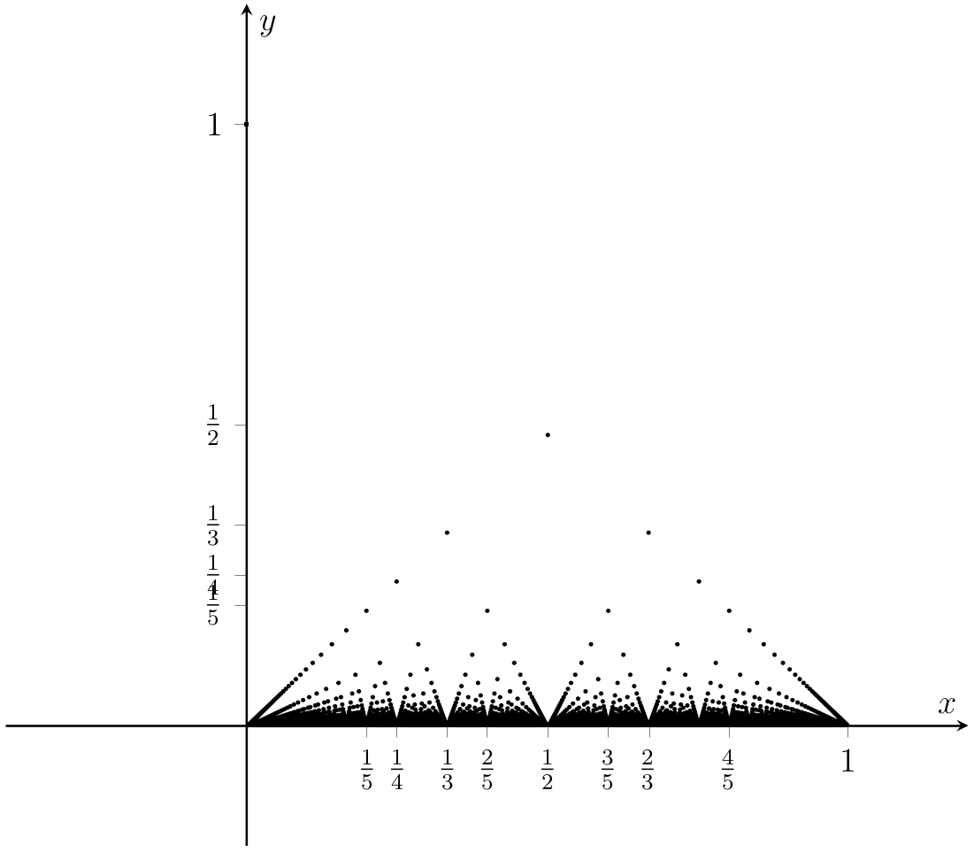
_images/dof.png — Fig. 3.1 Dirichlet’s other function.#

Remark 3.4

The function from Fig. 3.1 is also sometimes called Thomae’s function.

3.3. Continuity on closed bounded intervals#

We shall see in this section that functions that are continuous on closed bounded intervals are particularly well-behaved.

Many well-known functions have this property, including polynomials, sines, cosines and exponential functions. It turns out, as we will see, that there are some very important and powerful theorems that can be proved in this context.

The “main” theorems of this chapter all live in this section.

3.3.1. The intermediate value theorem#

Theorem 3.4 (The intermediate value theorem)

Let $f:[a,b]\to\mathbb{R}$ be continuous with $f(a) \neq f(b)$. Then for each $\gamma$ lying between $f(a)$ and $f(b)$, there exists $c \in (a, b)$ with $f(c) = \gamma$.

Proof. We prove Proposition 3.1 below, which is the special case where $\gamma=0$.

For the full result, apply Proposition 3.1 to the function $g(x):=f(x)-\gamma$ — see Problem 24. $\square$

Proposition 3.1 (Special case of the intermediate value theorem)

Let $f:[a,b]\to\mathbb{R}$ be continuous with $f(a) \neq f(b)$, and assume $f(a)$ and $f(b)$ have different signs. Then there exists $c \in (a, b)$ with $f(c) = 0$.

Proof. We only consider the case $f(b)<0<f(b)$, as the argument in the other case is so similar. We first construct a sequence $([a_{n}, b_{n}])$ of (nested) intervals satisfying the following properties:

(i) $[a_{n}, b_{n}] \subseteq [a_{n-1}, b_{n-1}]$, for all $n\in\mathbb{N}$,

(ii) $b_{n} - a_{n} = 2^{-n}(b - a)$, for all $n\in\mathbb{N}$,

(iii) $f(a_{n}) > 0, f(b_{n}) < 0$, for all $n\in\mathbb{N}$.

To do this we proceed as follows. Take $[a_{0}, b_{0}] = [a, b]$.

Now construct the interval $[a_{1}, b_{1}]$ as follows. Let $m_{1} = \frac{(a+ b)}{2}$. If $f(m_{1}) = 0$, then take $c = m_{1}$ and the theorem is proved. Otherwise, define

\[\begin{split} [a_{1}, b_{1}] = \begin{cases} [a, m_{1}] &\text{if $f(m_{1}) < 0$,}\\[.5em] [m_{1}, b] & \text{if $f(m_{1}) > 0$.} \end{cases} \end{split}\]

It is easily seen that (i), (ii) and (iii) all hold when $n =1$.

Now assume that we have constructed $[a_{1}, b_{1}], \ldots, [a_{n}, b_{n}]$ satisfying (i), (ii) and (iii). Let $m_{n+1} = \frac{(b_{n}+ a_{n})}{2}$. If $f(m_{n+1}) = 0$ then take $c = m_{n+1}$ and the theorem is proved. Otherwise define

\[\begin{split} [a_{n+1}, b_{n+1}] = \begin{cases} [a_{n}, m_{n+1}] &\text{if $f(m_{n+1}) < 0$,}\\[.5em] [m_{n+1}, b] & \text{if $f(m_{n+1}) > 0$.} \end{cases} \end{split}\]

By construction (i) and (iii) hold and for (ii) we have

\[ b_{n+1} - a_{n+1} = \frac{1}{2}(b_{n} - a_{n}) = \frac{1}{2}.2^{-n}(b -a) = 2^{-(n+1)}(b - a). \]

So by induction, the required sequence of intervals is constructed. Furthermore:

$(a_{n})$ is a monotonic increasing sequence and bounded above (by $b$),
$(b_{n})$ is a monotonic decreasing sequence and bounded below (by $a$).

By the monotone convergence theorem (MAS107 Theorem 3.10), both sequences converge, and by algebra of limits and (ii):

\[ \lim_{n\rightarrow\infty} b_{n} - \lim_{n\rightarrow\infty} a_{n} = \lim_{n\rightarrow\infty} 2^{-n}(b - a) = 0. \]

Define $c = \lim_{n\rightarrow\infty} b_{n} = \lim_{n\rightarrow\infty} a_{n}$. Then $c \in [a, b]$. By construction, we know that for all $n\in\mathbb{N}$, $f(a_n)>0$ and $f(b_n)<0$. Therefore, by continuity of $f$,

\[ f(c) = \lim_{n\rightarrow\infty} f(a_{n}) \geq 0 \hspace{2em} \text{ and } \hspace{2em} f(c) = \lim_{n\rightarrow\infty} f(b_{n}) \leq 0. \]

Hence $f(c) = 0$. As both $f(a)$ and $f(b) \neq 0$, $c \notin \{a, b\}$, i.e. $c \in (a, b)$. $\square$

Note that Theorem 3.4 tells us that the image (or range) of the interval $[a, b]$ under the continuous function $f$ contains the interval $[f(a), f(b)]$, i.e. $[f(a), f(b)] \subseteq f([a, b])$.

The next example gives a nice application of analysis to the theory of equations.

Example 3.12

Prove that every polynomial of odd degree has at least one real root.

Of course, there is no analogue of Example 3.12 when $m$ is even, e.g. $p(x) = x^{2} + 1$ has no real roots.

3.3.2. The extreme value theorem#

Definition 3.7 (Bounded function)

A function $f: X \rightarrow \mathbb{R}$ is bounded on a non-empty set $S \subseteq X$ if there exists $K > 0$, such that $|f(x)| \leq K$ for all $x \in S$.

In this situation, the set $\{f(x) : x \in S\}$ is a non–empty bounded set of real numbers and so, by completeness, it has a supremum, which we write as $\sup_{x \in S} f(x)$, and an infimum, which we write as $\inf_{x \in S}f(x)$.

Definition 3.8 (Attains its bounds)

We say that $f:X\to\mathbb{R}$ attains its bounds on $S\subseteq X$ if there exist $a, b \in S$ such that

\[ f(a) = \sup_{x \in S}f(x), \qquad f(b) = \inf_{x \in S}f(x). \]

Examples of functions $f:\mathbb{R}\to\mathbb{R}$ that are bounded on $\mathbb{R}$ are $f(x) = \sin(x)$ and $f(x) = \cos(x)$. Both functions attain their bounds, e.g. $f(x) = \sin(x)$ has supremum $1$ and this is attained at all points of the form $(4n + 1)\pi/2$, where $n \in \mathbb{Z}$; similarly the infimum $-1$ is attained at all points of the form $(4n - 1)\pi/2$, where $n \in \mathbb{Z}$.

We are interested in the case where $S$ is an interval and $f$ is continuous. The function $f(x) = \frac{1}{x}$ is continuous on the interval $(0, 1)$, but it is not bounded as it diverges to infinity at $0$. The function $f(x) = x$ is clearly bounded on $(0, 1)$, but it does not attain its bounds. When we restrict to closed intervals, we have a very nice result.

Theorem 3.5 (The extreme value theorem)

If $f:[a,b]\to\mathbb{R}$ is continuous, then it is bounded on $[a, b]$ and it attains its bounds there.

Proof. We first show that $f$ is bounded. To do this, we’ll assume that it isn’t, and seek a contradiction. So assume $f$ is not bounded. Let $(x_{n})$ be a sequence in $[a, b]$ such that

(3.1)#\[|f(x_{n})|\geq n \hspace{1em}\text{ for each }n\in\mathbb{N}.\]

Such a sequence certainly exists. For example, to construct such a sequence, we can consider $X_n=\{x \in [a, b] : |f(x)| \geq n\}$. This is non-empty since $f$ is unbounded and it is bounded below by $a$, so it has an infimum, say $x_{n} = \inf(X_n)$. And then $|f(x_{n})|\geq n$.

Now since $(x_{n})$ is a bounded sequence (as $a \leq x_{n} \leq b$, for all $n\in\mathbb{N}$), it has a convergent subsequence $(x_{n_{k}})$ by the Bolzano–Weierstrass theorem[2]. Let $x = \lim_{k \rightarrow \infty}x_{n_{k}}$. By continuity, $f(x) = \lim_{k \rightarrow \infty}f(x_{n_{k}})$. The sequence $(f(x_{n_{k}})))$ converges, and so in particular it must be bounded. But this contradicts our assumption (3.1).

Having proved that $f$ is bounded on $[a, b]$, we’ll prove that it attains its least upper bound. We again argue by seeking a contradiction. Let $\beta = \sup_{x \in [a, b]}f(x)$ and suppose that $\beta > f(x)$ for all $x \in [a, b]$. Then we can define $g: [a,b]\to\mathbb{R}$ by

\[ g(x) = \displaystyle\frac{1}{\beta - f(x)}, \]

and $g$ is continuous on $[a, b]$ by Theorem 3.2. By the first part of this current theorem, $g$ is bounded on $[a, b]$, so there exists $K > 0$ such that

(3.2)#\[g(x) \leq K \hspace{1em} \text{ for all } x \in [a, b].\]

The set $A=\{f(x) : x \in [a, b]\}$ is nonempty, and bounded above since $f$ is bounded. Therefore, for any $\varepsilon>0$, there exists $a\in A$ such that $a>\sup(A)-\varepsilon$. In particular, putting $\varepsilon = 1/K$, there exists $f(x) \in A$ such that $f(x) > \beta - 1/K$. But then $\beta - f(x) < 1/K$, and so $g(x) > K$, contradicting (3.2).

The argument for the greatest lower bound is similar, and is left for you as Problem 27. $\square$

It’s important to be clear what Theorem 3.5 is telling us. It says nothing about boundedness on $\mathbb{R}$. Indeed any non-constant polynomial is unbounded on $\mathbb{R}$, but its restriction to every closed interval $[a, b]$ is bounded.

Corollary 3.1 (Really useful corollary)

If $f: X \to \mathbb{R}$ is continuous and non–constant on $[a, b] \subseteq X$, then there exists $m < M$ so that

\[ f([a, b]) = [m, M]. \]

Proof. By Theorem 3.5, there exist $\gamma, \delta \in [a, b]$ such that $f(\gamma) = \inf_{x \in [a, b]}f(x)$ and $f(\delta) = \sup_{x \in [a, b]}f(x)$. We take $m = f(\gamma)$ and $M = f(\delta)$. Clearly, $m\leq M$ and, since $f$ is non-constant, $m<M$. If $x \in [a,b]$, then $f(x) \in [m, M]$ and so $f([a, b]) \subseteq [m, M]$.

For the other inclusion, by Theorem 3.4, given any $c \in (m, M)$ there exists $y \in (\gamma, \delta)$ (or in $(\delta, \gamma)$ depending on which number is smallest) so that $c = f(y)$, and it follows that $[m, M] \subseteq f([\gamma, \delta]) \subseteq f([a, b])$. $\square$

Remark. Corollary 3.1 says that continuous functions map closed bounded intervals to closed bounded intervals. The converse of this is false! For a counterexample, consider the function

\[\begin{split} f:\mathbb{R}\to\mathbb{R}; \hspace{1em} f(x) = \begin{cases} \sin\left(\frac{1}{x}\right) &\text{if }x \in \mathbb{R} \setminus \{0\},\\ 0&\text{if }x= 0. \end{cases} \end{split}\]

This function has the intermediate value property: the restriction of $f$ to any closed bounded interval $[a,b]\subseteq\mathbb{R}$ has image a closed bounded interval. However, $f$ is not continuous at $0$ (see Problem 9).

3.3.3. Inverses#

Let $X$ and $Y$ be arbitrary sets and $f:X \to Y$ be a function. Recall from MAS106 that $f$ is

surjective if the image of $f$ is equal to $Y$, i.e.~for all $y \in Y$ there exists $x \in X$ such that $f(x) = y$,
injective if whenever $f(x_{1}) = f(x_{2})$ for some $x_{1}, x_{2} \in X$, then $x_{1} = x_{2}$.
bijective if it is both surjective and injective.
invertible if there exists a function $f^{-1}: B \rightarrow X$, called the inverse of $f$, for which

\[ f^{-1}(f(x)) = x,~\mbox{for all}~x \in X~\mbox{and}~f(f^{-1}(y)) = y,~\mbox{for all}~y \in Y . \]

In the first year, you also saw the following.

Proposition 3.2

The function $f:X\rightarrow Y$ is invertible if and only if it is bijective.

When studying sequences in MAS107, you also encountered the notion of monotonicity: a sequence $(a_n)$ of real numbers is monotonic increasing if $a_n\leq a_m$ whenever $n<m$. It is monotic decreasing if $a_n\geq a_m$ whenever $n<m$, and a similar definition exists for monotonic descreasing sequences.

We now extend this idea to functions $f:X\to \mathbb{R}$ where $X\subseteq \mathbb{R}$.

Definition 3.9 (Monotone functions)

Let $f:X\to \mathbb{R}$ where $X\subseteq \mathbb{R}$.

We say that $f$ is

monotonic increasing if whenever $x, y \in X$ with $x < y$, we have $f(x) \leq f(y)$,
monotonic decreasing if whenever $x, y \in X$ with $x < y$, we have $f(x) \geq f(y)$,
monotone if it is either monotonic increasing or decreasing,
strictly monotonic increasing/decreasing when the $\leq$ or $\geq$ in the above definitions is replaced with $<$ or $>$ (respectively).

Note. It is standard practice to suppress the term “monotonic” and just describe a function as increasing or decreasing.

Here are some simple examples; it is easy to see that $f:\mathbb{R}\to\mathbb{R}$ given by $f(x) = x$ is strictly increasing, and that $f:(0,\infty) \to\mathbb{R}$ given by $f(x) = \frac{1}{x}$ is strictly decreasing. (So is $f:(-\infty, 0) \to\mathbb{R}$ given by $f(x) = \frac{1}{x}$, but not $f(x) = \frac{1}{x}$ on all of $\mathbb{R}\setminus\{0\}$).

Our key theorem considers the invertibility of monotone functions that are continuous on closed intervals.

Theorem 3.6 (The inverse function theorem)

If $f: [a,b] \rightarrow \mathbb{R}$ is continuous and strictly increasing (respectively, strictly decreasing), then $f$ is invertible and $f^{-1}$ is strictly increasing on $[f(a), f(b)]$ (respectively, strictly decreasing on $[f(b), f(a)]$) and continuous on $[f(a), f(b)]$ (respectively, on $[f(b), f(a)]$).

Proof. We’ll just consider the case where $f$ is strictly increasing. The argument for $f$ strictly decreasing is very similar.

By Corollary 3.1, the range of $f$ is of the form $[m, M]$, so $f:[a, b] \rightarrow [m, M]$ is surjective. Note that as $f$ is increasing, $m = f(a)$ and $M = f(b)$. If $x, y \in [a, b]$ with $x < y$ then $f(x) < f(y)$, so if $x \neq y$ then $f(x) \neq f(y)$. Hence $f$ is injective[3]. So $f$ is bijective, and hence invertible by Proposition 3.2. So we have $f^{-1}:[f(a), f(b)]\to [a,b]$.

To show that $f^{-1}$ is strictly increasing, let $f(a) \leq \alpha < \beta \leq f(b)$. Then since $f$ is surjective and increasing, there exist $a \leq x < y \leq b$ with $\alpha = f(x)$ and $\beta = f(y)$. Hence

\[ f^{-1}(\alpha) = f^{-1}(f(x)) = x < y = f^{-1}(f(y)) = f^{-1}(\beta). \]

Next we establish continuity of $f^{-1}$ at every $y_{0} \in (f(a), f(b))$. So given any $\varepsilon > 0$, we must find $\delta > 0$ such that $y \in (f(a), f(b))$ for which $|y_{0} - y| < \delta$ implies that $|f^{-1}(y) - f^{-1}(y_{0})| < \varepsilon$. Let $x_{0} = f^{-1}(y_{0})$, then $a < x_{0} < b$. Now for given $\varepsilon > 0$, choose $a < x_{1} < x_{0} < x_{2} < b$ such that $\max\{x_{2} - x_{0}, x_{0} - x_{1}\} < \varepsilon$. Let $y_{1} = f(x_{1})$ and $y_{2} = f(x_{2})$. Then since $f$ is strictly increasing,

\[ f(a) < y_{1} < y_{0} < y_{2} < f(b), \]

and if $y \in (y_{1}, y_{2})$ we have $|f^{-1}(y) - f^{-1}(y_{0})| < \varepsilon$. Then let $\delta = \min\{y_{2} - y_{0}, y_{0} - y_{1}\}$, and check that the $\varepsilon-\delta$ criterion is satisfied.

Finally, we leave continuity of $f^{-1}$ at $f(a)$ and at $f(b)$ as an exercise. $\square$

Example 3.13 ($n$th roots)

Fix $n\in\mathbb{N}$ and let $f:[0,\infty)\to[0,\infty)$ be given by $f(x) = x^n$. Then you can prove in Problem 31 that $f$ is strictly monotonic increasing on every $[a, b] \subseteq [0, \infty)$. We already know that $f$ is continuous.

Consider the restriction $f:[a,b]\to [a^n, b^n]$. By Theorem 3.6, to see that we have an inverse $f^{-1}: [a^n, b^n]\to [a,b]$ which is continuous and strictly monotonic increasing. Since we can do this for all intervals $[a,b]$, this allows us to obtain the function $[0, \infty)\to [0,\infty)$ that we write as $f(x)= x^{\frac{1}{n}}$.

So in particular, Theorem 3.6 has given us a unified method for proving the existence of positive $n$th roots of any positive real number.

Example 3.14

In Chapter 5, we’ll prove that $f:\mathbb{R}\to (0, \infty)$ given by $f(x) = e^{x}$ is monotonic increasing, as well as showing it is continuous. By a similar argument to that of Example 3.13, we can deduce that it has a continuous, monotonic increasing inverse $f^{-1}:(0, \infty)\to\mathbb{R}$. Of course, in this case $f^{-1}(x) =\ln(x) $ (or $\log_{e}(x)$, if you prefer) and so we are using Theorem 3.6 to deduce that every positive real number has a natural logarithm.