Revision of MAS107

1. Revision of MAS107#

This module will build directly on the work you have done in MAS107. In particular, it is important that you can recall definitions and results about sequences of real numbers, as we will be using them in many of the proofs and problems to come. When reviewing lecture notes before and after classes, it may help to have a copy of your MAS107 notes to hand, so that you can refresh any details that you need.

Unlike the other chapters in these notes, this chapter is intended as a summary and will not be lectured explicitly. Instead, I will do my best to take adequate time to recall any necessary concepts as we go.

Preliminary problems

This chapter is intended to be used in tandem with the Preliminary problems from the problem booklet. Ideally, you should aim to complete these problems during the first week or so of teaching[1].

Sometimes, the memory of being able to do something (e.g. last May, just before your MAS107 exam) can trick you into believing you are still able to do it. Tackling the problems will help you to tell the difference.

Don’t put this off: brushing up early on will make the learning to come much easier.

And remember, if you have any issues about this work or anything else from the module, myself and your other tutors are here to help — see 0.5. Where to get help for options. We’ve all been there and you won’t be judged.

1.1. Sequences and convergence#

Definition 1.1 (Convergent sequence)

A real sequence $(x_n)$ is said to converge to a limit $L\in\mathbb{R}$ if for all $\varepsilon>0$ there exists a number $N\in\mathbb{N}$[^office]: For in person, you can book an appointment, but don’t have to. such that

\[ |x_n-L| < \varepsilon \hspace{2em} \text{ for all } n\geq N. \]

In other words, for any given tolerance $\varepsilon$, the numbers $x_n$ will eventually all lie within $\varepsilon$ of $L$.

If $(x_n)$ converges to $L$, we write $\lim_{n\rightarrow}x_n=L$, or equivalently, $x_n\rightarrow L$ as $n\rightarrow\infty$.

One drawback of Definition 1.1 is that you need to have an idea of what the limit $L$ of the sequence might be, before getting started with the proof. The idea of a Cauchy sequence sometimes gets around this, so long as you are careful what set the sequence and limit belong to.

Definition 1.2 (Cauchy sequence)

A real sequence $(x_n)$ is called Cauchy if for all $\varepsilon>0$ there is an $N\in\mathbb{N}$ such that

\[ |x_n-x_m|<\varepsilon \hspace{2em} \text{ for all } m,n\geq N. \]

The key difference between Definition 1.1 and Definition 1.2 is what terms are being bounded by $\varepsilon$.

In Definition 1.1, terms in the sequence are getting closer and closer to a limit $L$. In Definition 1.2, terms of the sequence are getting closer and closer to one another, and no limit is mentioned.

In fact, being convergent within a given set is strictly stronger than being Cauchy: if $A\subseteq\mathbb{R}$ and $(x_n)$ is a sequence in $A$, then

\[\begin{split} (x_n) \text{ converges to a limit $L\in A$ } \hspace{1em} \substack{\Large\Rightarrow\\\Large\nLeftarrow} \hspace{1em} (x_n) \text{ is a Cauchy sequence in $A$}. \end{split}\]

The converse statement doesn’t hold: $(x_n)$ being Cauchy does not imply that it converges to a limit in $A$.

Example 1.1 (Cauchy sequence not converging in a given set $A$)

Let $A:=(0,1)$ and $x_n=\frac{1}{n}$, for $n\in\mathbb{N}$. Then, viewed as a sequence in $A$, $(x_n)$ does not converge. However, if we instead view it as a sequence in $\mathbb{R}$, we know that $x_n\rightarrow 0$ as $n\rightarrow\infty$. Since $(x_n)$ converges as a sequence in $\mathbb{R}$, it must be a Cauchy sequence.

Definition 1.3 (Complete subsets of $\mathbb{R}$)

A set $A\subseteq\mathbb{R}$ is called complete if every Cauchy sequence in $A$ converges to a limit in $A$.

Therefore, for complete sets, being Cauchy is equivalent to convergence. The set $\mathbb{Q}$ of all rational numbers is not complete, but the set $\mathbb{R}$ of all reals is.

In Example 1.1, we saw that $(0,1)$ is not a complete set, because it does not contain the limit of the sequence $x_n=\frac{1}{n}$.

Exercise: Prove that $\mathbb{Q}$ is not complete. That is, find a sequence $(x_n)$ of rational numbers converging to an irrational limit. Then, prove this sequence is Cauchy.

In MAS107, you saw how $\mathbb{R}$ is constructed from $\mathbb{Q}$ by including the limits of all rational Cauchy sequences.

1.2. Logic and quantifiers#

Analysis, like all areas of pure mathematics, is interested in proving things carefully and rigorously. This requires technical arguments, and in order to communicate unambiguously, we will need to use formal language such as quantifiers.

There are two important quantifiers used by mathematicians:

Universal quantifier: $\forall$, “for all”
Existential quantifier: $\exists$ “there exists”

Understanding mathematical statements involving quantifiers takes continual practice. A key advantage of studying analysis is there will be plenty of opportunity for this.

Example 1.2

Definition 1.1 can be expressed more succincly using quantifiers:

\[ x_n\rightarrow l \; \text{ iff } \;\forall\varepsilon>0\; \exists N\in\mathbb{N} \;\text{ s.t. }\forall n\geq N\; |x_n-l|<\varepsilon. \]

In words:

“$x_n$ converges to $l$ if and only if for all $\varepsilon>0$, there exists $N\in\mathbb{N}$ such that for all $n\geq N$ we have $|x_n-l|<\varepsilon$”.

Exercise: Express Definition 1.2 in terms of quantifiers.

1.2.1. Negation#

The negation of a mathematical statement is its logical opposite. When negating statements involving quantifiers, the roles of $\forall$ and $\exists$ trade places, while all other parts of the statement are replaced with their logical opposites.

For example, consider the definition of disjoint sets.

\[ A, B\subseteq\mathbb{R} \; \text{ are disjoint \; iff }\;\; \forall x\in A, \; x\notin B. \]

The negation is

\[ A, B\subseteq\mathbb{R} \; \text{ are }\textbf{not}\text{ disjoint iff }\;\; \exists x\in A, \text{ s.t } x\in B. \]

For an example involving longer statements, consider again the definition of convergence:

\[ x_n\rightarrow l \; \text{ iff } \;\forall\varepsilon>0\; \exists N\in\mathbb{N} \;\text{ s.t. }\forall n\geq N\; |x_n-l|<\varepsilon. \]

The negation of this is

\[ x_n\not\rightarrow l \; \text{ iff } \;\exists\varepsilon>0\; \;\text{ s.t. }\forall N\in\mathbb{N} \;\exists n\geq N\;\;\text{ s.t. } |x_n-l|\geq\varepsilon. \]

That is, $x_n\not\rightarrow l$ if and only if there is some $\varepsilon>0$ for which, no matter how large we choose $N$, there is an even larger $n$ for which $|x_n-l|\geq\varepsilon$. You can think of this as “$|x_n-l|\geq\varepsilon$ infinitely often”.

1.3. Inequalities#

Inequalities are the primary tool of analysts. Here is a reminder of the two most important ones for this module (and beyond).

1.3.1. The triangle inequality#

Theorem 1.1

For all real numbers $a$ and $b$,

\[ |a+b| \leq |a|+|b|. \]

Proof. The proof involves splitting into cases according to the signs $a$ and $b$. When $a$ and $b$ have the same sign, we get equality $|a+b|=|a|+|b|$.

Otherwise, suppose (without loss of generality) that $a<0<b$, so that $|a|+|b|=b-a$. For the other side, either $|a+b|=a+b=|b|-|a|$, or $|a+b|=-a-b=|a|-|b|$. Both of these are clearly less than $|a|+|b|$.$\square$

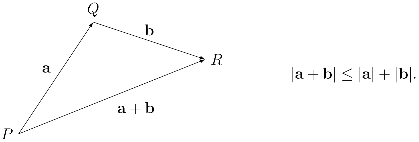
Note that the triangle inequality holds in higher dimensions, too. If $\textbf{a}$ and $\textbf{b}$ are vectors in $\mathbb{R}^n$, then the vectors $\mathbf{a}$, $\mathbf{b}$ and $\mathbf{a}+\mathbf{b}$ form sides of a triangle.

If the vertices of this triangle are $P$, $Q$ and $R$, then the triangle inequality is just saying that it is a shorter distance to walk from $P$ to $R$ directly than it would be to walk there via the point $Q$.

$Triangle with vertices $P$, $Q$ and $R$, and edges $\overrightarrow{PQ}=\mathbf{a}$, $\overrightarrow{QR}=\mathbf{b}$ and $\overrightarrow{PR}=\mathbf{a}+\mathbf{b}$. It is always shorter to travel directly from $P$ to $R$ than it is to go via $Q$. In other words, $|\mathbf{a}+\mathbf{b}|\leq|\mathbf{a}|+|\mathbf{b}|$.$

The following corollary of the triangle inequality will also be frequently useful.

Corollary 1.1

For all $a,b\in\mathbb{R}$,

\[ \Big||a|-|b|\Big| \leq |a-b|. \]

Proof. Since the statement is symmetric in $a$ and $b$, we can assume without loss of generality that $|a|>|b|$. By the triangle inequality,

\[ |a| = |(a-b) +b| \leq |a-b| +|b|, \]

and so

\[ |a|-|b|\leq |a-b|. \]

Since we’re assuming $|a|>|b|$,

\[ \Big||a|-|b|\Big| \leq |a|-b|, \]

and so we are done. $\square$