6. Riemann integration — Non-examinable 2024–25

In this chapter we will go over the rigorous definition of the integral, defined in terms of area beneath curves. You have seen the idea before in MAS106, but now we can make it precise using limits.

6.1. Partitions and Riemann sums

Let \([a,b]\subseteq\mathbb{R}\) be a closed bounded interval. A partition of \([a,b]\) refers to any finite subset \(P=\{x_0,x_1,\ldots,x_n\}\) of \([a,b]\) that contains the endpoints \(a\) and \(b\). For such a partition, it is convenient to assume that

\[ a=x_0<x_1<x_2<\ldots<x_n=b. \]

Let \(f:[a,b]\to\mathbb{R}\) be a bounded function. For each partition \(P\) of \([a,b]\), we associate two ways of approximating the area under the graph of \(f\) by rectangles. One of these ways will always be an overestimate, the other an underestimate.

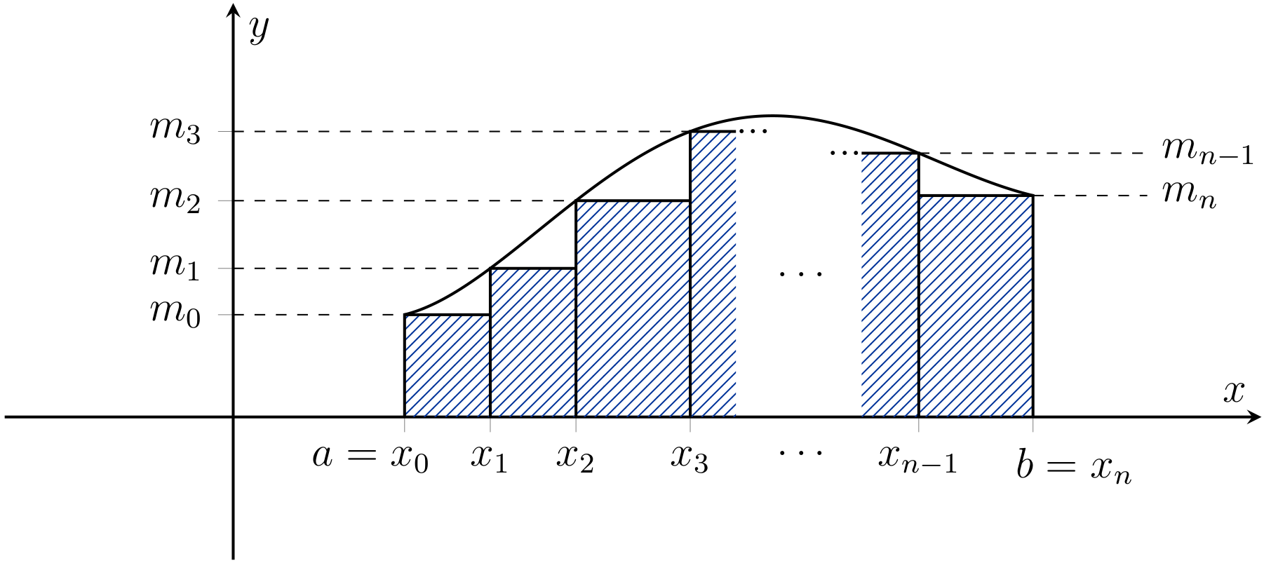
Fig. 6.1 Riemann lower sum

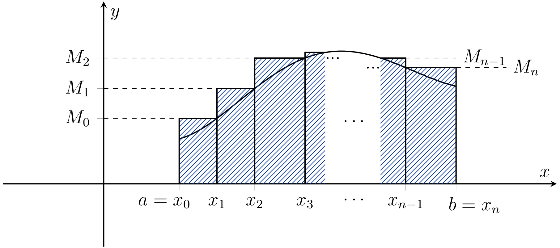
Fig. 6.2 Riemann upper sum

Definition 6.1 (Upper and lower sums)

Let \(f:[a,b]\to\mathbb{R}\) be a bounded function, and let \(P=\{x_0,x_q,\ldots,x_n\}\) be a partition.

For \(k=1,\ldots,n\) let

\[ m_k=\inf\{f(x) : x\in[x_{k-1},x_k]\} \hspace{1em} \text{and} \hspace{1em} M_k=\sup\{f(x) : x\in[x_{k-1},x_k]\}. \]

The sum

\[ L(f,P) := \sum_{k=1}^nm_k(x_k-x_{k-1}) \]

is called the (Riemann) lower sum of \(f\) with respect to \(P\), and

\[ U(f,P) := \sum_{k=1}^nM_k(x_k-x_{k-1}) \]

is the (Riemann) upper sum of \(f\) with respect to \(P\).

For both the upper and lower sum, the widths of the rectangles are the same: they are determined by the partition \(P\). It is the heights of the rectangles that provide the distinction: for the lower sum, the heights \(m_k\) are determined by taking the infimum of \(f\) over each interval \([x_{k-1},x_k]\) (see Fig. 6.1). For the upper sum, heights \(M_k\) are obtained by taking the supremum of \(f\) over each of these intervals (c.f. Fig. 6.2).

Example 6.1

Let \(f:[-1,5]\to\mathbb{R}\); \(f(x)=3x^2+1\) and \(P=\{-1,1,2,5\}\). Calculate \(L(f,P)\), \(U(f,P)\) and \(U(f,P)-L(f,P)\).

Solution (click for drop down)

In the notation of Definition 6.1, we have \(m_1=\inf\{3x^2+1 : x\in[-1,1]\}=1\), \(m_2=\inf\{3x^2+1 : x\in[1,2]\}=4\), and \(m_3=\inf\{3x^2+1:x\in[2,5]\}=13\).

Therefore,

\[ L(f,P) := \sum_{k=1}^nm_k(x_k-x_{k-1}) = 1(2) + 1(1) + 13(3) = 42. \]

On the other hand, \(M_1=\sup\{3x^2+1 : x\in[-1,1]\}=4\), \(M_2=\sup\{3x^2+1 : x\in[1,2]\}=13\), \(M_3=\sup\{3x^2+1:x\in[2,5]\}=76\). Hence

\[ U(f,P) := \sum_{k=1}^nM_k(x_k-x_{k-1}) = 4(2) + 13(1) + 76(3) = 249. \]

Hence \(U(f,P)-L(f,P)=207\).

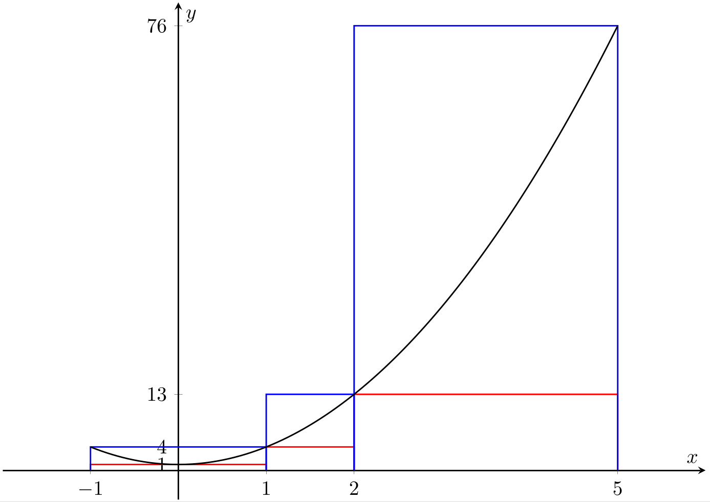
Fig. 6.3 Riemann upper and lower sums for Example 6.1.

The lower sums \(L(f,P)\) are always an under-approximation for the (signed) area between \(f\) and the \(x\) axis, while the upper sums \(U(f,P)\) always over-approximate this area.

In particular, \(L(f,P)<U(f,Q)\) for any two partitions \(P\) and \(Q\) of \([a,b]\), with the true value of the signed area under \(f\) lying somewhere between these two values.

We introduce the notion of refinement of partitions, which will be useful for proving properties of the Riemann integral.

Definition 6.2 (Refinement of a partition)

Let \(P\) and \(Q\) be partitions of \([a,b]\). We say that \(Q\) is a refinement of \(P\) if \(P\subseteq Q\).

Lemma 6.1

Let \(f:[a,b]\to\mathbb{R}\) and let \(P\) and \(Q\) be partitions of \([a,b]\). If \(Q\) is a refinement of \(P\), then

\[ L(f,Q) \geq L(f,P) \text{ and } U(f,Q)\leq U(f,P). \]

In particular,

\[ U(f,Q)-L(f,Q)\leq U(f,P)-L(f,P). \]

Proof. Let \(P=\{x_0,x_1,\ldots,x_n\}\) where \(a=x_0<x_1<\ldots<x_n=b\). Consider first the effect of adding one point to \(P\): say we add \(c\in[x_{k-1},x_k]\). We will show that \(L(f,P\cup\{c\})\geq L(f,P)\).

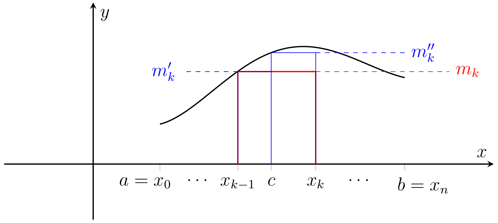
Fig. 6.4 The effect of adding a point to a partition

Let \(\;\displaystyle m_k = \inf_{x\in[x_{k-1},x_k]}f(x)\), \(\;\displaystyle m_k' = \inf_{x\in[x_{k-1},c]}f(x)\), and \(\;\displaystyle m_k'' = \inf_{x\in[c,x_k]}f(x)\).

Observe that \(m_k'\geq m_k\) and \(m_k''\geq m_k\). This is because \(m_k\) is the infimum of \(f(x)\) taken over the whole of \([x_{k-1},x_k]\), while \(m_k'\) and \(m_k''\) are infima taken over subintervals \([x_{k-1},c]\) and \([c,x_k]\). Therefore,

\[\begin{align*} L(&f,P\cup\{c\}) \\ &= m_0(x_1-x_0) + \ldots + m_k'(c-x_{k-1}) + m_k''(x_k-c) + \ldots + m_n(x_n-x_{n-1}) \\ &\geq m_0(x_1-x_0) + \ldots + m_k(c-x_{k-1}) + m_k(x_k-c) + \ldots + m_n(x_n-x_{n-1}) \\ &= m_0(x_1-x_0) + \ldots + m_kc-m_kx_{k-1} + m_kx_k-m_kc + \ldots + m_n(x_n-x_{n-1}) \\ &= m_0(x_1-x_0) + \ldots + m_k(x_k-x_{k-1}) + \ldots + m_n(x_n-x_{n-1}) \\ &= L(f,P). \end{align*}\]

Applying a similar argument to the upper sums shows that

\[ U(f,P\cup\{c\})\leq U(f,P). \]

Finally, suppose \(Q\) is a refinement of \(P\). Since \(Q\setminus P\) is finite, we can apply the above argument recursively to prove that \(L(f,Q)\geq L(f,P)\) and \(U(f,Q)\leq U(f,P)\). \(\square\)

Remark 6.1

Lemma 6.1 is saying that refining a partion has the effect of shrinking the difference between the upper and lower sums. This fact will be essential in proofs to come!

6.2. The Riemann integral

We are now ready to define the Riemann integral.

Let \(f:[a,b]\to\mathbb{R}\) be a bounded function, and consider the set of all lower sums

\[ S_L:=\{L(f,P):\text{ partitions } P \text{ of } [a,b]\}. \]

This is a set of real numbers. It is certainly non-empty: we can take \(P=\{a,b\}\), then \(m_1=\min\{f(a),f(b)\}\), and \(L(f,P)=m_1(b-a)\in S_L\). \(S_L\) is also bounded above by the area we have been trying to calculate. This means we can take its supremum.

By an analogous argument, the set of all upper sums

\[ S_U:=\{U(f,P):\text{ partitions } P \text{ of } [a,b]\}. \]

is non-empty and bounded below. So we can take its infimum.

Definition 6.3 (Upper and lower integrals)

The lower integral of \(f\) is

\[ L(f) = \sup S_L = \sup\{L(f,P):\text{ partitions } P \text{ of } [a,b]\}. \]

The upper integral of \(f\) is defined to be

\[ U(f) = \inf S_U = \inf\{U(f,P):\text{ partitions } P \text{ of } [a,b]\}. \]

The lower and upper integrals exist for any bounded function on \([a,b]\), though they may not be equal to each other. However, it is always the case that

\[ L(f) \leq U(f), \]

since \(L(f,P)<U(f,Q)\) for any two partitions \(P\) and \(Q\) of \([a,b]\).

Definition 6.4

We say that a bounded function \(f:[a,b]\to\mathbb{R}\) is Riemann integrable if \(L(f)=U(f)\). In this case, we write

\[ \int_a^b f(x)dx := L(f) = U(f). \]

Example 6.2 (Constant functions)

Suppose that \(f:[a,b]\to\mathbb{R}\) is a constant function; say \(f(x)=C\) for all \(x\in[a,b]\). Then for any partition \(P=\{x_0,\ldots,x_n\}\), where \(a=x_0<x_1<\ldots<x_n=b\),

\[ M_k=\sup_{x\in[x_k,x_{k-1}]}f(x) = C \]

and

\[ m_k=\inf_{x\in[x_k,x_{k-1}]}f(x) = C. \]

Therefore

\[ L(f,P) = U(f,P) = \sum_{k=1}^nC(x_k-x_{k-1}) = C(x_n-x_0)=C(b-a). \]

It follows that \(L(f)=U(f)=C(b-a)\), and hence \(f\) is integrable, with

\[ \int_a^bf(x)dx=\int_a^bCdx=C(b-a). \]

The following is a handy criterion for proving that more sophisticated functions are integrable.

Proposition 6.1 (Integrability criterion)

A bounded function \(f:[a,b]\to\mathbb{R}\) is integrable if and only if the following criterion holds:

For all \(\varepsilon>0\), there is a partition \(P_\varepsilon\) such that \(U(f,P) - L(f,P) < \varepsilon\).

Proof. (\(\Leftarrow\)) Observe that for any partition \(P\) of \([a,b]\),

\[ 0\leq U(f)-L(f) \leq U(f,P)-L(f,P). \]

Therefore, if the criterion holds, it follows that

\[ 0\leq U(f)-L(f) <\varepsilon, \]

for any \(\varepsilon>0\). Hence \(U(f)=L(f)\), and so \(f\) is Riemann integrable.

(\(\Rightarrow\)) Conversely, if \(f\) is Riemann integrable, then we know that \(\int_a^b f(x)dx = L(f)=U(f)\). By definition of \(L(f)\) and \(U(f)\), given \(\varepsilon>0\), we can find partitions \(P\) and \(Q\) of \([a,b]\) such that

\[ L(f,P) > L(f) - \frac{\epsilon}{2}, \]

and

\[ U(f,Q) < U(f) + \frac{\epsilon}{2}. \]

Note that the union \(P\cup Q\) is a refinement of both \(P\) and \(Q\). By Lemma 6.1,

\[\begin{align*} U(f,P\cup Q) - L(f,P\cup Q) &\leq U(f,Q) - L(f,P) \\ &\leq U(f) + \frac{\epsilon}{2} - (L(f) - \frac{\epsilon}{2}) = \epsilon. \end{align*}\]

\(\square\)

Example 6.3

Consider \(f(x)=\left\{\begin{array}{cl} 1 & \text{ if } x < 1 \\ 2 &\text{ if } x \geq 1. \end{array}\right.\) on the interval \([0,2]\).

Prove \(f\) is integrable, and calculate \(\int_0^2f(x)dx\).

Solution (click for drop down)

Let’s first draw the graph of \(f\) and employ some intuition.

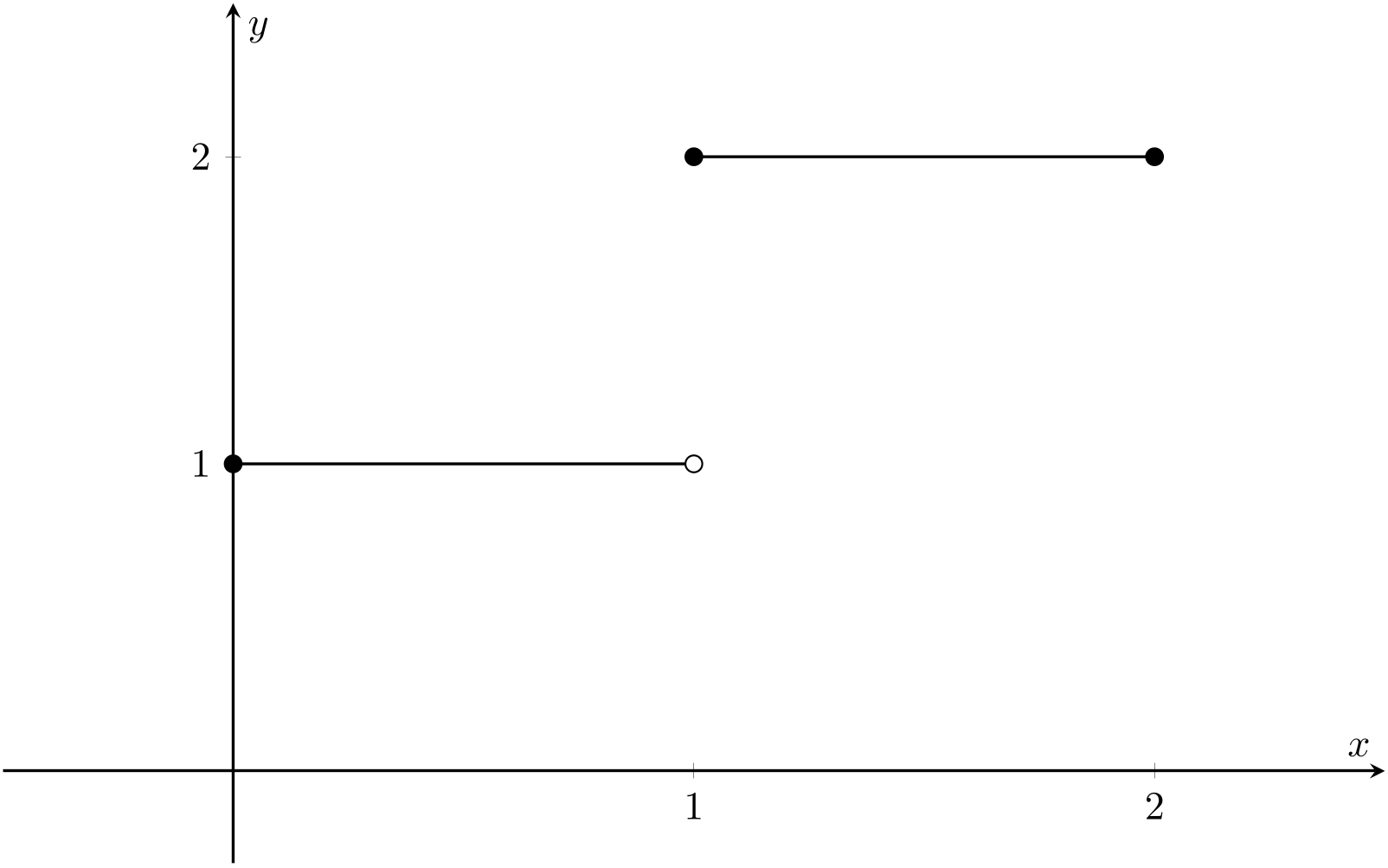
Fig. 6.5 Graph of \(f\).

The graph suggests we should find that \(\int_0^2f(x)dx=L(f)=U(f)=3\).

We can prove this intuition is correct using Proposition 6.1. Let \(\varepsilon>0\). We seek a partition \(P_\varepsilon\) of \([0,2]\) such that

\[ U(f,P_\varepsilon)-L(f,P_\varepsilon)<\varepsilon \]

Let’s try and find a partition of the form \(P_\varepsilon=\{0,1-\delta,1+\delta,2\}\), where \(\delta\) is to be found and depends on \(\varepsilon\).

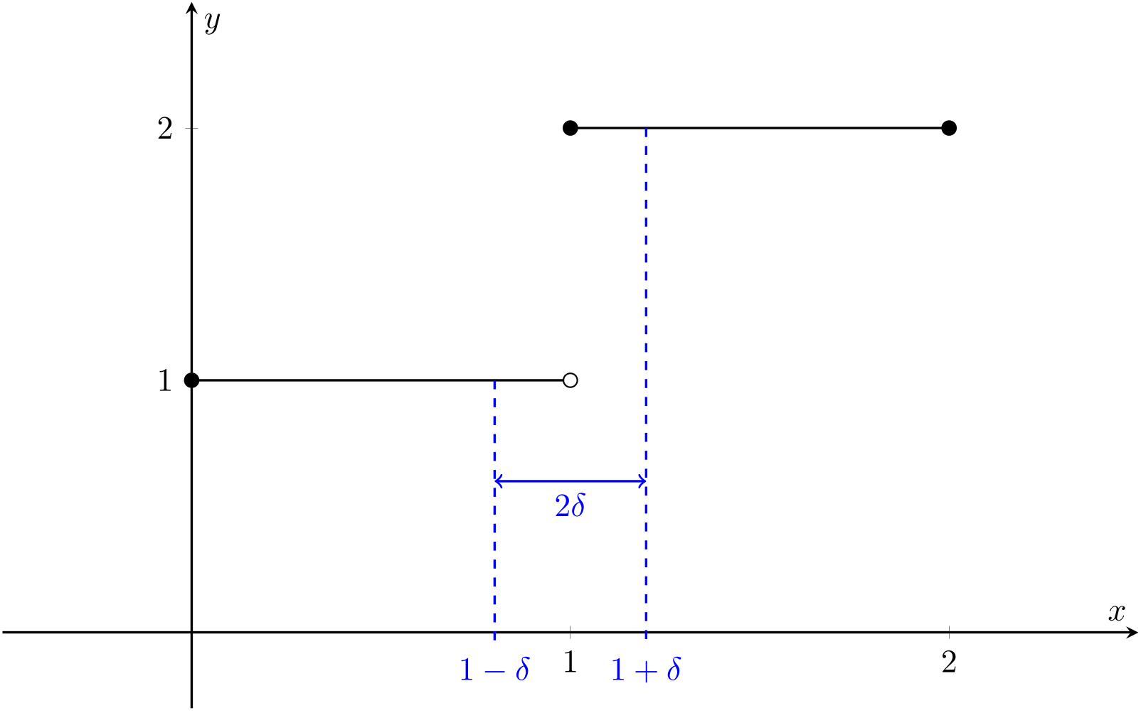
Fig. 6.6 Partition of the form \(P_\varepsilon=\{0,1-\delta,1+\delta,2\}\).

We could take a guess of what we need to make \(\delta\), but it will be much easier to do so after calculating \(U(f,P_\varepsilon)-L(f,P_\varepsilon)\).

We have \(m_1=\inf\{f(x):x\in[0,1-\delta]\}=1\), \(m_2=\inf\{f(x):x\in[1-\delta,1+\delta]\}=1\) and \(m_3=\inf\{f(x):x\in[1+\delta,2]\}=2\).

Hence, using Definition 6.1,

\[ L(f,P_\varepsilon)= 1\cdot(1-\delta)+1\cdot(2\delta) + 2(2-(1+\delta)) = 1+\delta+2-2\delta = 3-\delta. \]

By a similar calculation, \(M_1=\sup\{f(x):x\in[0,1-\delta]\}=1\), \(m_2=\sup\{f(x):x\in[1-\delta,1+\delta]\}=2\) and \(m_3=\sup\{f(x):x\in[1+\delta,2]\}=2\).

\[ U(f,P_\varepsilon)=1\cdot(1-\delta)+2\cdot(2\delta)+2\cdot(2-(1+\delta)) = 1-\delta+4\delta+2-2\delta = 3+\delta. \]

So, $\( U(f,P_\varepsilon)-L(f,P_\varepsilon) = 3+\delta - (3-\delta) = 2\delta. \)$

Therefore, if we take \(\delta:=\frac{\epsilon}{2}\), (and so \(P_\varepsilon = \left\{0,1-\frac{\varepsilon}{2},1+\frac{\varepsilon}{2},2\right\}\)), Proposition 6.1 is satisfied, and thus \(f\) is integrable.

Moreover, by properties of sup, for all \(\varepsilon>0\),

\[ U(f)\leq U(f,P_\varepsilon) = 3+\frac{\varepsilon}{2}. \]

So \(U(f)\leq 3\). And by properties of inf, for all \(\varepsilon>0\),

\[ L(f)\geq L(f,P_\varepsilon)=1-\frac{\varepsilon}{2}, \]

So \(L(f)\geq 3\). But also, since \(f\) is integrable, \(L(f)=U(f)\leq 3\). The only option is

\[ \int_0^2f(x)dx = U(f) = L(f) = 3. \]

Phew!

In Example 6.3, we successfully integrated a discontinuous function. An 18th century mathematician could never!

In a similar vein, we have the following.

Proposition 6.2 (Integrating indicator functions)

Let \(a,b\in\mathbb{R}\) with \(a<b\). Then \(\mathbb{1}_{[a,b]}\), \(\mathbb{1}_{[a,b]}\), \(\mathbb{1}_{[a,b]}\) and \(\mathbb{1}_{[a,b]}\) are all Riemann intervagrable on \([a,b]\), with

\[ \int_a^b\mathbb{1}_{[a,b]}(x)dx = \int_a^b\mathbb{1}_{(a,b)}(x)dx = \int_a^b\mathbb{1}_{[a,b)}(x)dx = \int_a^b\mathbb{1}_{(a,b]}(x)dx = b-a. \]

Proof. For \(\mathbb{1}_{[a,b]}\), this is just a special case of Example 6.2, and there is nothing to show. The rest is for you to do as Problem 68.

As another application of Proposition 6.1, we can prove that all monotone functions defined on a closed bounded interval are integrable.

Theorem 6.1

Let \(f:[a,b]\to\mathbb{R}\) be a monotone function. Then \(f\) is integrable.

Proof. Assume for simplicity that \(f\) is monotone increasing. The proof for monotone decreasing functions is very similar.

Let \(P=\{x_0,x_1,\ldots,x_n\}\) be a partition of \([a,b]\), where \(a=x_0<x_1<\ldots<x_n=b\) as before. Then since \(f\) is increasing, for all \(1\leq k\leq n\)

\[ M_k = \sup_{x\in[x_{k-1},x_k]}f(x) = f(x_k), \]

and

\[ m_k = \inf_{x\in[x_{k-1},x_k]}f(x) = f(x_{k-1}). \]

Therefore,

(6.1)\[\begin{split}\begin{aligned} U(f,P) - L(f,P) &= \sum_{k=1}^nf(x_k)(x_{k-1}-x_k) - \sum_{k=1}^nf(x_{k-1})(x_{k-1}-x_k) \\ &= \sum_{k=1}^n\big(f(x_k)-f(x_{k-1})\big)(x_{k-1}-x_k). \end{aligned}\end{split}\]

This is true for any partition \(P\). Let \(\varepsilon>0\). We aim to choose a partition \(P\) in such a way that \(U(f,P) - L(f,P)<\varepsilon\); the result will then follow by Proposition 6.1.

Let \(P\) be the partition with points

\[ x_k=a+\left(\frac{b-a}{n}\right)k, \hspace{2em} \text{ for } k=0,1,\ldots,n. \]

That, is \(P\) divides \([a,b]\) into \(n\) equal pieces. In particular, \(x_k-x_{k-1}=\frac{b-a}{n}\) for each \(k\).

By equation (6.1),

\[ U(f,P) - L(f,P) = \frac{b-a}{n}\sum_{k=1}^n\big(f(x_k)-f(x_{k-1})\big) \]

This is a telescopic sum, and when written out, most of the terms cancel. We get

\[ U(f,P)-L(f,P) = \frac{b-a}{n}\big(f(x_n)-f(x_0)\big) = \frac{b-a}{n}\big(f(b)-f(a)\big) \]

(since \(x_0=a\) and \(x_n=b\)).

Proving the condition from Proposition 6.1 is now simply a matter of choosing \(n\) sufficiently large so that

\[ \frac{b-a}{n}\big(f(b)-f(a)\big) < \varepsilon. \]

Any integer larger than \(\displaystyle\frac{(b-a)(f(b)-f(a))}{\varepsilon}\) will suffice. \(\square\)

Another large class of integrable functions is the continuous functions on closed bounded intervals. Unfortunately there is not sufficient time in this module to cover its proof, though the general approach is not disimilar to Theorem 6.1. A non-examinable proof can be found in the appendix for interest.

Theorem 6.2

Let \(f:[a,b]\to \mathbb{R}\) be continuous. Then \(f\) is Riemann integrable.

In case we are tempted to think that all functions are integrable, here is an example of a non-integrable function.

Example 6.4 (A non-integrable function)

Define \(f:[0,1]\rightarrow \mathbb{R}\) by

\[\begin{split} f(x) = \left\{ \begin{array}{lll} 0 & x\in \mathbb{Q}, \\ 1 & x\not\in \mathbb{Q}. \\ \end{array} \right. \end{split}\]

Show that \(f\) is not Riemann integrable.

Solution. We show that \(U(f)\neq L(f)\), by direct calculation. Let \(P=\{x_0,x_1,\ldots,x_n\}\) be a partition of \([0,1]\), and assume as usual that \(0=x_0<x_1<\ldots<x_n=1\).

Note that every interval, however small, contains both rational and irrational numbers. This means that

\[ M_k = \sup_{x\in[x_{k-1},x_k]}f(x) = 1 \hspace{1em} \text{ and } \hspace{1em} m_k = \inf{x\in[x_{k-1},x_k]}f(x) = 0 \]

for \(k=1,\ldots,n\). But then

\[ U(f,P) = \sum_{k=1}^n(x_k-x_{k-1}) = x_n-x_0 = 1, \]

while \(L(f,P)=0\). Taking \(\sup\)’s and \(\inf\)’s over all partitions \(P\) of \([0,1]\), it follows that \(U(f)=1\) and \(L(f)=0\). So \(U(f)\neq L(f)\), and \(f\) is not Riemann integrable.

6.3. Properties of the integral

We gather together some useful properties of the Riemann integral. Those that are not proven directly here will be proven in the problem booklet.

Proposition 6.3

Let the bounded functions \(f,g:[a,b]\rightarrow \mathbb{R}\) be Riemann integrable.

(i) Suppose \(f(x)\leq g(x)\) for all \(x\in [a,b]\). Then

\[ \int_a^b f(x)dx \leq \int_a^b g(x)dx. \]

(ii) Let \(f:[a,b]\to\mathbb{R}\) be bounded, and let \(c\in [a,b]\). If \(f\) is integrable, then so is the restriction of \(f\) to \([a,c]\) and \([c,b]\), and

\[ \int_a^b f(x)dx = \int_a^cf(x)dx + \int_c^bf(x)dx. \]

Conversely, if \(f\) is integrable on \([a,c]\) and \([c,b]\) then it is integrable on \([a,b]\).

(iii) Let \(\alpha ,\beta \in \mathbb{R}\). Then \(\alpha f+ \beta g:[a,b]\to\mathbb{R}\) is Riemann integrable and

\[ \int_a^b\big(\alpha f(x) + \beta g(x)\big)dx = \alpha \int_a^b f(x)dx + \beta \int_a^b g(x)dx. \]

(iv) The function \(|f|:[a,b]\to \mathbb{R}\); \(x\mapsto|f(x)|\) is Riemann integrable, and

\[ \left| \int_a^b f(x)dx \right| \leq \int_a^b |f(x)|dx. \]

Proof. (i) Since \(f\) is integrable, we have \(\int_a^b f(x)dx = U(f) = \inf\{U(f,P):P\text{ a partition of }[a,b]\}\). Therefore

\[ \int_a^b f(x)dx \leq U(f,P) \]

for any partition \(P\) of \([a,b]\). Also, since \(f(x)\leq g(x)\) for all \(x\in[a,b]\), it is easy to check that \(U(f,P)\leq U(g,P)\). Hence

\[ \int_a^b f(x)dx \leq U(g,P) \]

for all partitions \(P\) of \([a,b]\). Taking the infimum over \(P\),

\[ \int_a^b f(x)dx \leq U(g) = \int_a^bg(x)dx, \]

since \(g\) is integrable.

(ii) Let \(f|_{[a,c]}\) denote the restriction of \(f\) to \([a,c]\), and \(f|_{[c,b]}\) the restriction of \(f\) to \([c,b]\).

We first show that

\[ U(f) = U(f|_{[a,c]})+U(f|_{[c,b]}) \hspace{.5em} \text{and}\hspace{.5em} L(f) = L(f|_{[a,c]})+L(f|_{[c,b]}). \]

Let \(P_1\) be any partition of \([a,c]\) and \(P_2\) be any partition of \([c,b]\). Then \(P:=P_1\cup P_2\) is a partition of \([a,b]\). One can check by writing out the Riemann sums explicitly that

\[ U(f,P) = U(f|_{[a,c]},P_1)+U(f|_{[c,b]},P_2). \]

and

\[ L(f,P) = L(f|_{[a,c]},P_1)+L(f|_{[c,b]},P_2). \]

Therefore

(6.4)\[U(f) \leq U(f|_{[a,c]},P_1)+U(f|_{[c,b]},P_2),\]

and

(6.5)\[L(f) \geq L(f|_{[a,c]},P_1)+L(f|_{[c,b]},P_2)\]

Taking the infimum in (6.4) first over \(P_1\) and then over \(P_2\) gives

(6.4)\[U(f) \leq U(f|_{[a,c]})+U(f|_{[c,b]}).\]

Similarly, taking the supremum in (6.5), first over \(P_1\) and then over \(P_2\),

(6.5)\[L(f) \geq L(f|_{[a,c]})+L(f|_{[c,b]}).\]

On the other hand, if \(P\) now denotes any partition of \([a,b]\), then by Lemma 6.1,

\[ U(f,P) \geq U(f,P\cup\{c\}). \]

Let \(P_1=\Big(P\cup\{c\}\Big)\cap[a,c]\) and \(P_2=\Big(P\cup\{c\}\Big)\cap[c,b]\). Then \(P_1\) is a partition of \([a,c]\), \(P_2\) is a partition of \([c,b]\), and \(P\cup\{c\} = P_1\cup P_2\). Hence,

\[ U(f,P) \geq U(f,P\cup\{c\}) = U(f,P_1) + U(f,P_2) \geq U(f|_{[a,c]}) + U(f_{[c,b]}). \]

Taking \(\inf\)’s over \(P\), we have \(U(f) \geq U(f|_{[a,c]})+U(f|_{[c,b]})\), which when combined with (6.4) gives

\[ U(f) = U(f|_{[a,c]})+U(f|_{[c,b]}). \]

A similar argument applied to the lower sums shows that \(L(f) \leq L(f|_{[a,c]})+L(f|_{[c,b]})\), and so by (6.5),

\[ L(f) = L(f|_{[a,c]})+L(f|_{[c,b]}). \]

Finally, observe that we can now write

\[ 0\leq U(f) - L(f) = \Big(U(f|_{[a,c]}) - L(f|_{[a,c]})\Big) + \Big(U(f|_{[c,b]}) - L(f|_{[c,b]}\Big), \]

and each of these two brackets are greater than or equal to zero. It follows that \(U(f)=L(f)\) if and only if \(U(f|_{[a,c]}) = L(f|_{[a,c]})\) and \(U(f|_{[c,b]}) = L(f|_{[c,b]}\). That is, \(f\) is integrable if and only if \(f|_{[a,c]}\) and \(f|_{[c,b]}\) are both integrable. If this is the case, then

\[ \int_a^b f(x)dx = U(f) = U(f|_{[a,c]}) + U(f|_{[c,b]}) = \int_a^cf(x)dx+\int_c^bf(x)dx. \]

(iii) See Problems 70 and 71.

(iv) Since \(-|f(x)|\leq f(x) \leq |f(x)|\) for all \(x\in[a,b]\) the result will follow from part (i) if we can show that \(|f|\) is integrable. This is for you to do as Problem 72.\(\square\)

Proposition 6.3(ii) is particularly useful as it allows us to integrate functions with a finite number of jump discontinuities, by splitting its domain into intervals on which it is continuous.

Example 6.5

Consider the step function

\[ s:[0,4] \rightarrow \mathbb{R}; \; s(x) = \mathbf{1}_{[2,3]}(x)-\mathbf{1}_{[0,2)}(x)+2\mathbf{1}_{(3,4]}(x). \]

Show that \(s\) is integrable and calculate \(\int_0^4s(x)dx\).

Solution (click for drop down)

Using the definition of an indicator function, we have

\[\begin{split} s(x) = \left\{\begin{array}{cc} -1 & \text{if } 0\leq x<2 \\ 1 & \text{if } 2\leq x\leq 3 \\ 2 & \text{if } 3< x\leq 4 \end{array}\right. \end{split}\]

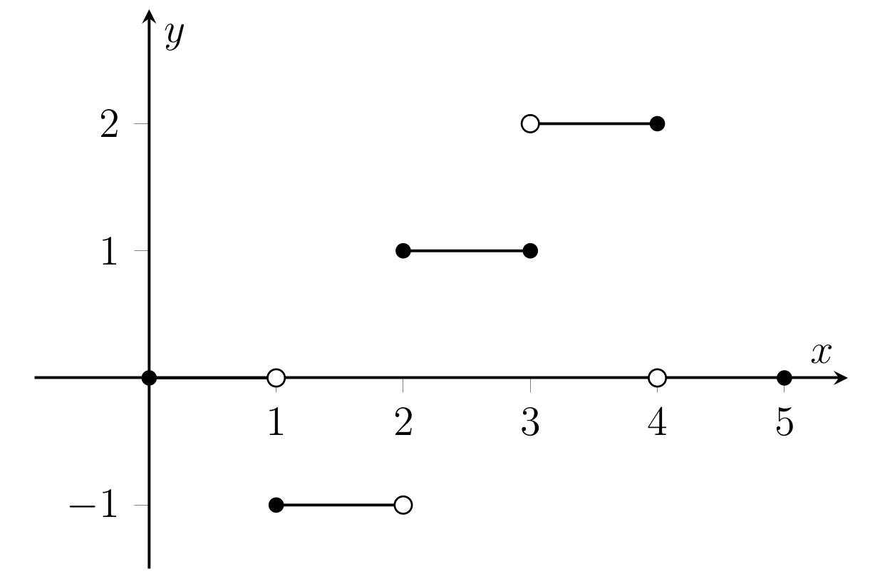
Fig. 6.7 Graph of the step function \(s\).

Direct inspection of the graph of \(s\) indicates that

\[ \int_0^2s(x)dx=-2,\; \int_2^3s(x)dx=1, \; \text{ and } \; \int_3^4s(x)dx=2. \]

Hence by Proposition 6.3(ii),

\[ \int_0^4s(x)dx = \int_0^2s(x)dx + \int_2^3s(x)dx + \int_3^4s(x)dx = -2 + 1 + 2 = 1. \]

Exchanging limits in an integral

Technically, we have only defined \(\int_a^bf(x)dx\) when \(a<b\).

Definition 6.5

For an integrable function \(f:[a,b]\to\mathbb{R}\), we define

\[ \int_b^af(x)dx = -\int_a^bf(x)dx, \]

and

\[ \int_a^af(x)dx=0. \]

Definition 6.5 is a natural convention that mainly serves the purpose of simplifying the algebra of integrals. Importantly, it does not disturb the validity of any part of Proposition 6.3.

6.4. The fundamental theorem of calculus

So far, integration has exclusively referred to area calculation. In this section we link it with the reverse of differentiation. This is known as the fundamental theorem of calculus. You are already familiar with this statement, but now we are in a position to give a full proof.

We first need a quick lemma.

Lemma 6.2

Let the bounded function \(f:[a,b]\rightarrow \mathbb{R}\) be Riemann integrable. Let

\[ m = \inf \{ f(x) : x\in [a,b] \}, \qquad M = \sup \{ f(x) : x\in [a,b] \}. \]

Then

\[ m(b-a) \leq \int_a^b f(x)dx \leq M(b-a). \]

Proof. Consider the partition \(P=\{a,b\}\) of \([a,b]\). The associated Riemann sums are

\[ L(f,P) = m(b-a) \hspace{1em} \text{ and } \hspace{1em} U(f,P) = M(b-a). \]

Since \(f\) is integrable,

\[ \int_a^b f(x)dx = L(f) \geq m(b-a), \]

and

\[ \int_a^b f(x)dx = U(f) \leq M(b-a). \]

\(\square\)

Theorem 6.3 (Fundamental theorem of calculus)

Let \(f:[a,b]\rightarrow \mathbb{R}\) be continuous. Define \(F:[a,b]\rightarrow \mathbb{R}\) by

\[ F(x) = \int_a^x f(t)dt. \]

Then \(F\) is differentiable, and \(F'(x) = f(x)\) for all \(x\in [a,b]\).

Proof. Note first that \(F\) is well defined: by Theorem 6.2, \(f\) is integrable.

Let \(h>0\) and let \(x\in [a,b]\). Then, using Proposition 6.3(ii),

\[ F(x+h)-F(x) = \int_a^{x+h} f(t) dt -\int_a^{x} f(t) dt = \int_x^{x+h} f(t) dt. \]

In other words, \(F(x+h)-F(x)\) is the area under the curve between \(x\) and \(x+h\).

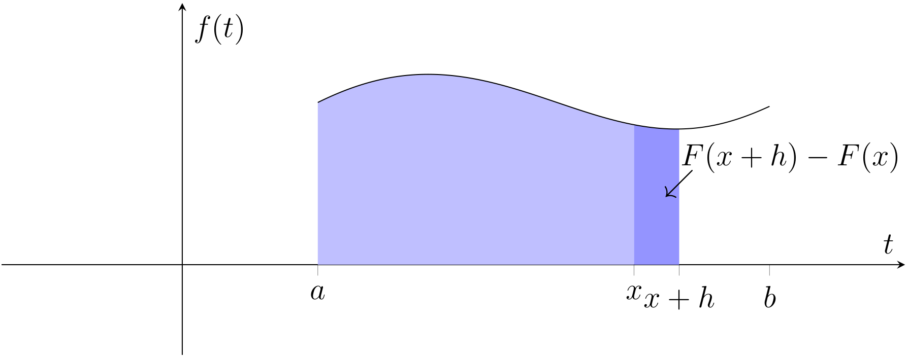
Fig. 6.8 Visualisation of \(F(x+h)-F(x)\).

Since \(f\) is continuous, by the extreme value theorem (Theorem 3.5) it is bounded on \([x,x+h]\) and attains its bounds. That is,

\[ f(c_h) = \inf \{ f(t) : t\in [x,x+h ] \}, \hspace{1em} \text{ and } \hspace{1em} f(k_h) = \sup \{ f(t) : t\in [x,x+h] \}, \]

for some \(c_h,k_h\in[x,x+h]\). Therefore, by Lemma 6.2,

\[F hf(c_h) \leq F(x+h) - F(x) \leq h\cdot f(k_h), \]

and so

(6.6)\[f(c_h)\leq \frac{F(x+h)-F(x)}{h} \leq f(k_h). \]

The same inequality holds when \(h<0\); the proof is similar.

Since \(c_h,k_h\in[x,x+h]\) for all \(h\), we have \(c_h, k_h\rightarrow 0\) as \(h\rightarrow 0\). Therefore, by continuity of \(f\) at \(x\),

\[ \lim_{h\rightarrow 0} f(c_h) = \lim_{h\rightarrow 0} f(k_h) = f(x). \]

Applying the squeeze theorem to (6.6),

\[ \lim_{h\rightarrow 0} \frac{F(x+h)-F(x)}{h} = f(x). \]

That is, \(F\) is differentiable at \(x\) and \(F'(x) =f(x)\). \(\square\)

The version of the theorem that we use in practice to calculate integrals follows as a corollary.

Corollary 6.1

Let \(f:[a,b]\rightarrow \mathbb{R}\) be a continuous function. Suppose we have a differentiable function \(F:[a,b]\to \mathbb{R}\) such that \(F'(x) =f(x)\) for all \(x\in [a,b]\). Then

\[ \int_a^b f(t)dt = F(b) - F(a). \]

Proof. Let \(G:[a,b]\to \mathbb{R}\) be given by

\[ G(x) = \int_a^x f(t)dt. \]

Then \(G(a)=0\), and by Theorem 6.3, \(G\) is differentiable with

\[ G'(x) =f(x) =F'(x). \]

So we have a constant \(C\) such that \(G(x)=F(x)+C\) for all \(x\in [a,b]\). Now

\[\begin{align*} \int_a^b f(t)\ dt = G(b) &= G(b) - G(a) \\ &= (F(b)+C) - (F(a)+C) = F(b) -F(a). \end{align*}\]

\(\square\)

Note that all of the techniques we already know about finding integrals, such as substitution and integration by parts, can be proved for continuous functions with an ``antiderivative”, Theorem 4.3.