Limits of functions

2. Limits of functions#

2.1. Functions on the real line#

In this section, we revise some aspects of functions and look at some examples. This is mostly revision of material from MAS106.

We will be interested in functions $f:X\to Y$, where $X$ and $Y$ are some subsets of the real numbers $\mathbb{R}$ (perhaps the whole of $\mathbb{R}$). Recall that $f$ being a function from $X$ to $Y$ means that for each element $x\in X$, there is specified exactly one element $f(x)\in Y$, the value of the function $f$ on the element $x$.

The domain of $f$ is $X$, and we sometimes use the notation $\text{Dom}(f):=X$. The set $Y$ is called the codomain of $f$. The range (or image) of the function $f$ is the set

\[ \text{Range}(f)=\{y \in Y : y = f(x)~\mbox{for some}~x \in X\}; \]

that is, it is the set of values attained by the function.

It is important in this course that a function has a specified domain and codomain. In particular, giving a formula, like $\frac{1}{x}$, for example, is not giving a function, although it may be part of the information that specifies a function. We could give a function by, for example, saying $f:\mathbb{R}\setminus\{0\}\to \mathbb{R}$, given by $f(x)=\frac{1}{x}$. And this is a different function from $f:(0,1)\to \mathbb{R}$, also given by $f(x)=\frac{1}{x}$.

Notice that we have used the difference of sets notation here: recall that if $X$ and $Y$ are arbitrary sets, then

\[ X \setminus Y = X \cap Y^{c} = \{x \in X : x \notin Y\}. \]

If we have some formula in $x$ that we would like to use for the value $f(x)$ of a function, it is often useful to think about the largest domain $f$ could have, that is, the set of all $x$ in $\mathbb{R}$ for which $f(x)$ makes sense as a real number. This will not include any $x \in \mathbb{R}$ for which we might be tempted to write “$f(x) = 0/0$” or “$f(x) = \pm \infty$”.

2.2. Examples of functions#

2.2.1. Standard functions#

Example 2.1 (Polynomial functions)

A polynomial is a function $f:X\to\mathbb{R}$ of the form

\[ f(x) = a_{0} + a_{1}x + \cdots + a_{n-1}x^{n-1} + a_{n}x^{n}, \]

where the coefficients $a_{0}, a_{1}, \ldots, a_{n}$ are in $\mathbb{R}$, and the degree $n$ is a natural number. Here, $X$ can be any subset of $\mathbb{R}$.

Example 2.2 (Rational functions)

A rational function is a function $f:X\to\mathbb{R}$ of the form $f(x) = \frac{p(x)}{q(x)}$, where $p$ and $q$ are polynomials. The largest subset of $\mathbb{R}$ we can take as its domain $X$ is $\{x \in \mathbb{R} : q(x) \neq 0\}$.

For example, if $f(x) = \displaystyle\frac{x^{2} + 5}{(x+1)(x-3)}$, the largest possible domain of $f$ is $\mathbb{R} \setminus \{-1, 3\}$.

Example 2.3 (The sign function)

The sign function $\text{sgn}:\mathbb{R}\to \mathbb{R}$ is defined by

\[\begin{split} \text{sgn}(x) = \left\{\begin{array}{c c} -1 & ~\mbox{if}~x < 0,\\ 0 & ~\mbox{if}~x = 0,\\ 1& ~\mbox{if}~x > 0. \end{array} \right. \end{split}\]

The range of this function is $\{-1, 0, 1\}$.

Example 2.4 (Indicator functions)

If $S\subseteq\mathbb{R}$, then indicator function of $S$ is the function $\mathbb{1}_{[a,b]}:\mathbb{R}\to\mathbb{R}$ given by

\[\begin{split} \mathbb{1}_{S}(x) = \left\{\begin{array}{c c} 1 & ~\mbox{if}~x \in S,\\ 0& ~\mbox{if}~x \notin S. \end{array} \right. \end{split}\]

Indicator functions can look quite unremarkable if the set $S$ is something simple like an interval. Step functions can be built by taking linear combinations of indicator functions over different intervals — this will be useful when we study integration later on.

Other important functions are the functions $f:\mathbb{R}\to\mathbb{R}$, given by $f(x) = e^{kx}, f(x) = \sin(kx)$ and $f(x) = \cos(kx)$, where $k \in \mathbb{R}$. In analysis, they are best defined as convergent power series — see later.

2.2.2. Weird functions#

When learning analysis this semester, we will often take a general function $f:X\to\mathbb{R}$ and reason about it. It is very easy and natural to imagine quite a nice function for $f$ in such a situation — a nice smooth, bounded curve with (at worst) a finite number of jump discontinuities and no fractal structure. We know many functions that are like this, but statistically[1], most are not. General functions can be far stranger.

It’s important to remember we are developing a theory that needs to apply to all functions, not just the nice ones. Below are some examples of some of the weirder functions that we will study in weeks to come. If you know of any other weird functions, please let me know and I might include them.

Example 2.5 (Dirichlet’s function)

This is the name given to the indicator function $\mathbb{1}_\mathbb{Q}$. We will return to it several times to explore the nuances of limits and continuity (see Example 3.10). For now, I invite you to try drawing its graph.

Example 2.6 (Dirichlet’s other function.)

Also known as Thomae’s function. Let $g:[0,1)\to\mathbb{R}$ be defined by

\[\begin{split} g(x) =\begin{cases} 1 &\text{if $x = 0$},\\ \displaystyle\frac{1}{n}& \text{if $x = m/n \in \mathbb{Q}$, and $\text{hcf}(m,n)=1$}\\ 0&\text{if $x \in \mathbb{R} \setminus \mathbb{Q}$}. \end{cases} \end{split}\]

Try sketching this! Other names include: the popcorn function, the raindrop function, and the countable cloud function. I’ll let you sketch it to work out why.

Example 2.7 (Functions from Problems 9, 10, 41 and 42)

Consider the functions $\sin(1/x)$, $x\sin(1/x)$ and $x^2\sin(1/x)$. What do their graphs look like? Can they be defined meaningfully on the whole real line?

The final weird function of this section is a famous example of a everywhere continuous, nowhere differentiable function.

Its construction is less explicit than some of the other examples in this section, and in fact, since Weierstrass’ work, others have found more naturally-occuring examples of such functions (e.g. Brownian motion). However, this function is something of an icon, so we include it.

Example 2.8 (Weierstrass function)

Let $0<a<1$, let $b\in\mathbb{N}$ be odd, and such that $ab>1+\frac{3\pi}{2}$. It can be shown that $f:\mathbb{R}\to\mathbb{R}$; $f(x)=\sum_{n=0}^\infty a^n\cos\left(b^n\pi x\right)$ is a well-defined, continuous, and nowhere-differentiable function (this bit uses ideas to do with uniform convergence of infinite series — see Chapter 5).

https://upload.wikimedia.org/wikipedia/commons/6/60/WeierstrassFunction.svg — Fig. 2.1 Graph of the Weierstrass function. Image credit.#

We will return to many of these functions in our work to come.

2.3. Functional limits#

We want to make rigorous the notion of $\lim_{x \rightarrow a}f(x)$, for a function $f:X \rightarrow \mathbb{R}$, and a point $a\in\mathbb{R}$. Note that $a$ may not be an element of the domain $X$, here (though it can be). You have already studied this in MAS106 and you should have good intuition for this situation. Here we will make the idea precise, using sequences.

2.3.1. The $(\epsilon-\delta)$ definition#

First note that it only makes sense to consider the behaviour of $f(x)$ as $x\rightarrow a$ if there are points in the domain of $f$ that get arbitrarily close to $a$.

Definition 2.1 (Limit point)

Let $X\subseteq\mathbb{R}$. A real number $a$ is called a limit point of $X$ if there is a sequence $(x_n)$ in $X$ that converges to $a$ and satisfies $x_n\neq a$ for all $n\in\mathbb{N}$.

Equivalently, $a$ is a limit point of $X$ if any open interval containing $a$ has non-empty intersection with $X\setminus\{a\}$.

Example 2.9

(i) Let $X=(0,2)\cup\{3\}$. Then $0$ and $2$ are limit points of $X$, but $3$ is not.

(ii) A real number $a\in\mathbb{R}$ is a limit point of $[0,1]$ if and only if $a\in[0,1]$.

(iii) More generally, given $a<b$, then $[a,b]$ is the set of all limit points for any of the intervals $(a,b)$, $(a,b]$, $[a,b)$ and $[a,b]$.

Definition 2.2 (Functional limit)

Let $f:X\to\mathbb{R}$ be a function, let $a\in\mathbb{R}$ be a limit point of $X$, and let $l\in\mathbb{R}$.

We say that $f$ converges to $l$ as $x\rightarrow a$, and write

\[ \lim_{x \rightarrow a}f(x) =l, \]

if, for all $\varepsilon>0$ there exists $\delta>0$ such that for all $x\in X$,

\[ 0<|x-a|<\delta \; \text{ implies } \; |f(x)-l|<\varepsilon. \]

Notes.

We require that $a$ be a limit point of $X$ so that it to make sense to consider what happens to the values of the function as we approach $a$.
The real number $a$ may or may not be in the domain $X$.

Example 2.10

Let $f:(0,1)\to\mathbb{R}$ and suppose that

\[ f(x) = 5x+2. \]

Common sense tells us that $\lim_{x\rightarrow 1}f(x)=7$. Let’s try to prove this rigorously using Definition 2.2.

Let $\varepsilon>0$. We seek $\delta>0$ such that $0<|x-1|<\delta$ implies $|f(x)-7|<\varepsilon$. On the other hand,

\[ |f(x)-7| = |5x+2-7| = |5x-5| = 5|x-1| \]

This tells us that if we choose $\delta:=\frac{\varepsilon}{5}$, then

\[ 0<|x-1|<\delta \Rightarrow |f(x)-7|<5\delta=5\cdot\frac{\varepsilon}{5}=\varepsilon. \]

This proves that Definition 2.2 holds, and so $\lim_{x\rightarrow 1}f(x)=7$.

Definition 2.2 is usually referred to as the “$(\varepsilon-\delta)$ definition” of the functional limit, and does well to capture the idea of a limit is that as $x$ gets closer and closer to $a$, so $f(x)$ should get closer and closer to $l$.

2.3.2. Sequential criterion#

There is a second, equivalent definition for the limit of a function, in terms of limits of sequences of points in its domain. This sequential definition of limits is sometimes more useful in proofs, since we can use theorems already proven for convergence of sequences (see for example Theorem 2.2, coming up).

Theorem 2.1 (Sequential criterion for functional limits)

Let $f:X \rightarrow \mathbb{R}$, let $a\in\mathbb{R}$ be a limit point of $X$, and let $l\in\mathbb{R}$. The following are equivalent:

(i) $\lim_{x\rightarrow a} f(x) = l$.

(ii) (Sequential criterion) For every sequence $(x_n)$ in $X\setminus\{a\}$ with $\lim_{n\rightarrow\infty}x_n=a$, we have that $\lim_{n\rightarrow\infty}f(x_n) = l$.

Proof. (i)$\Rightarrow$(ii): Suppose $\lim_{x\rightarrow a} f(x) = l$, and suppose $\varepsilon > 0$. So there exists $\delta > 0$ such that for all $x \in X$,

\[ 0<|x - a| < \delta \Rightarrow |f(x) - l| < \varepsilon. \]

Let $(x_{n})$ be an arbitrary sequence in $X\setminus\{a\}$ with limit $a$. Then since $x_n\rightarrow a$, there exists $N\in\mathbb{N}$, such that $0<|x_{n} - a| < \delta$ for all $n\geq N$. But then, for all $n \geq N$, we have $|f(x_{n}) - l| < \varepsilon$, and so $\lim_{x\rightarrow a} f(x) = l$, as was required. We have established that $(i)\Rightarrow(ii)$.

(ii)$\Rightarrow$(i): Now we must establish the converse, namely that if $(x_n)$ is a sequence in $X\setminus\{a\}$ that converges to $a$, then the real sequence $(f(x_n))$ converges to $l$, as $n\rightarrow\infty$. We seek a proof by contradiction. Suppose that that $f(x)$ does not converge to $l$ as $x\rightarrow a$. Then the $(\varepsilon-\delta)$ criterion fails: there exists an $\varepsilon>0$ such that for all $\delta > 0$, there exists $x \in X$ with $0 < |x - a| < \delta$, but $|f(x) - l| \geq \varepsilon$.

Now for this $\varepsilon>0$, choose successively $\delta = 1, \frac{1}{2}, \frac{1}{3}, \ldots$ and construct a sequence $(x_{n})$ as follows:

\[\begin{split} x_{1} \in X \text{ satisfies } 0<|x_{1} - a| < 1 \text{ and }|f(x_{1}) - l| \geq \varepsilon. \\ x_{2} \in X\text{ satisfies } 0<|x_{2} - a| < \frac{1}{2}\text{ and }|f(x_{2}) - l| \geq \varepsilon.\\ \vdots x_{n} \in X\text{ satisfies }0<|x_{n} - a| < \frac{1}{n}\text{ and }|f(x_{n}) - l| \geq \varepsilon. \end{split}\]

Then $(x_n)$ is a sequence in $X\setminus\{a\}$ and by the squeeze theorem, we have $\lim_{n\rightarrow\infty} x_{n} = a$. Also, by the above construction the sequence $(f(x_{n}))$ does not converge to $l$.

So we have shown that if the $(\varepsilon-\delta)$ criterion fails, then so does the sequential criterion for functional limits. This completes the proof of Theorem 2.1. $\square$

Example 2.11

Consider the function from Example 2.10

\[ f:(0,1)\to\mathbb{R}; \; f(x) = 5x+2. \]

For any sequence $(x_n)$ in $(0,1)$ with $x_n\rightarrow 1$, we have

\[ f(x_n) = 5x_n+2 \rightarrow 7, \]

by algebra of limits for sequences. Therefore $\lim_{x\rightarrow 1}f(x)=7$.

Consider how much quicker this proof was, compaired with that of Example 2.10. The sequential criterion is often easier to apply in proofs about limits of functions.

2.3.3. Algebra of limits and the Squeeze[2] Theorem#

In MAS107, you proved many theorems concerning convergence of real sequences. Theorem 2.1 gives us a way to capitalise on this hard work and quickly arrive at results about limits of functions.

Reminder: Pointwise operations with functions.#

Let $X,Y\subseteq\mathbb{R}$, and let $f:X\to\mathbb{R}$ and $g:Y\to\mathbb{R}$ be functions. Let $\alpha\in\mathbb{R}$. We define new functions, $f+g$, $\alpha f$, $fg$ and $\frac{f}{g}$ pointwise, but we need to be careful with domains.

Pointwise sum.

\[ f+g:X\cap Y\to \mathbb{R}; \; (f+g)(x) := f(x) + g(x), \]

Pointwise scalar multiplication.

\[ \alpha f:X\to \mathbb{R}; \; (\alpha f)(x):=\alpha f(x), \]

Pointwise multiplication.

\[ fg: X\cap Y\to\mathbb{R}; \; (fg)(x):=f(x)g(x), \]

Pointwise division. Here, more care must be taken with domains:

\[ \frac{f}{g}:\left\{x\in X\cap Y:g(x)\neq 0\right\} \to\mathbb{R}; \; \left(\frac{f}{g}\right)(x) := \frac{f(x)}{g(x)}. \]

Remark 2.1

In each case, the domain is taken to be the largest subset of $\mathbb{R}$ for which the pointwise operation is defined.
MAS2004 students should recall from Semester 1 the set ${\cal F}(\mathbb{R})$ of all functions from $\mathbb{R}$ to $\mathbb{R}$. The pointwise operations of addition and scalar multiplication turn $\mathcal{F}$ into a vector space over $\mathbb{R}$ (but it is not finite-dimensional). Pointwise multiplication gives $\mathcal{F}(\mathbb{R})$ the additional structure of an algebra over $\mathbb{R}$. These structural properties are important in higher analysis (e.g. functional analysis).

Theorem 2.2 (Algebra of limits)

Suppose that $f:X \rightarrow \mathbb{R}$, $g :Y \rightarrow \mathbb{R}$, and $a \in \mathbb{R}$ is such that $\lim_{x\rightarrow a} f(x)$ and $\lim_{x\rightarrow a} g(x)$ both exist. Then

(i) $\displaystyle\lim_{x\rightarrow a} (f + g)(x) = \lim_{x\rightarrow a} f(x) + \lim_{x\rightarrow a} g(x)$,

(ii) $\displaystyle\lim_{x\rightarrow a} (fg)(x) = \left(\lim_{x\rightarrow a} f(x)\right)\left(\lim_{x\rightarrow a} g(x)\right)$,

(iii) $\displaystyle\lim_{x\rightarrow a} (\alpha f)(x) = \alpha \lim_{x\rightarrow a} f(x)$, for all $\alpha \in \mathbb{R}$,

(iv) $\displaystyle\lim_{x\rightarrow a} \left(\displaystyle\frac{f}{g}\right)(x) = \displaystyle\frac{\lim_{x\rightarrow a} f(x)}{\lim_{x\rightarrow a} g(x)}$, provided $\lim_{x\rightarrow a} g(x) \neq 0$.

In particular, the limits in (i)–(iv) all exist.

Proof. By Theorem 2.1, these all follow from the algebra of limits for sequences. For example, for (i), if $(x_{n})$ is an arbitrary sequence in $X\cap Y$ with $x_n\neq a$ for all $n\in\mathbb{N}$ such that $(x_n)$ that converges to $a$, then

\[\begin{align*} \lim_{n\rightarrow\infty} (f + g)(x_{n}) &= \lim_{n\rightarrow\infty} (f(x_{n}) + g(x_{n})) \\ &= \lim_{n\rightarrow\infty} f(x_{n}) + \lim_{n\rightarrow\infty} g(x_{n})\\ &= \lim_{x\rightarrow a} f(x) + \lim_{x\rightarrow a} g(x), \end{align*}\]

as required.

Here the first line uses the definition of a sum of functions and the second line uses algebra of limits (for real sequences). $\square$

The sequential condition for limits of functions is also usually easier to use when proving that a function does not converge to a finite limit. This is because we need only find one sequence in which the sequential condition fails.

Example 2.12

Consider $f:\mathbb{R} \setminus \{-5, 3, 5\}\to \mathbb{R}$, given by

\[ f(x) = \frac{x - 5}{(x^{2} - 25)(x - 3)}. \]

Investigate $\lim_{x \rightarrow a}f(x)$ for each $a\in\mathbb{R}$. (You will need to think about points in the domain and each of the three special points $-5, 3, 5$ separately.)

Solution: Note that for $x\in\mathbb{R} \setminus \{-5, 3, 5\}$,

(2.1)#\[f(x) = \frac{x - 5}{(x-5)(x+5)(x - 3)}= \frac{1}{(x+5)(x - 3)}.\]

Note that (2.1) does not hold at $x=-5,3$ or $5$, as $f(x)$ has not been defined there. We must use the definition of $f$ and its domain that we have been given, not what we might hope it could be.

Equation (2.1) is still useful for determining any limiting behaviour of $f$ at these points, however.

Let’s write $X=\mathbb{R}\setminus\{-5, 3, 5\}$, the domain of $f$. Note that every real number is a limit point of $X$. However, the most interesting limit points to consider are those that lie outside of $X$. This is because it is fairly easy to calculate limits at points in $X$.

For example, to calculate the limit at $x=1$: using (2.1) and algebra of limits (Theorem 2.2), we have $\lim_{x\rightarrow 1}(x+5) = 6$, $\lim_{x\rightarrow 1}(x-2)=-1$, and so

\[ \lim_{x \rightarrow 1}f(x) = \lim_{x\rightarrow 1}\frac{1}{(x+5)(x-3)} = \frac{1}{6(-2)}= -\frac{1}{12}=f(1). \]

More generally, in this example, if you take the limit at a point $a$ lying inside the domain $X$ of $f$, algebra of limits (Theorem 2.2) implies that

\[ \lim_{x\rightarrow a} f(x) = \lim_{x\rightarrow a}\frac{1}{(x+5)(x-3)} = \frac{1}{(a+5)(a-3)} = f(a). \]

This tells us that the function $f$ is continuous at these points. We will discuss the concept of continuity in more detail in Chapter 3.

The more interesting problem is to find out what happens at limits points that are not in $X$. Observe that

To investigate the point $x = 5$:
$5$ is a limit point of $X$, but does not lie inside $X$. However, since the formula $\frac{1}{(x+5)(x-3)$ is well-defined at $x=5$, the algebra of limits argument still works. We just have to be careful not to write “$f(5)$” anywhere, as $5\notin X$.

Alternative method using sequences: Choose an arbitrary sequence $(x_{n})$ with $x_{n} \in X$ satisfying $\lim_{n \rightarrow \infty}x_{n} = 5$.

Then $f(x_{n}) = \displaystyle\frac{1}{(x_{n}+5)(x_{n}-3)}$ and $\displaystyle\lim_{n \rightarrow \infty}f(x_{n}) = \displaystyle\frac{1}{10.2} = \displaystyle\frac{1}{20}$, by the algebra of limits. So we conclude that

\[ \lim_{x \rightarrow 5}f(x) = \frac{1}{20}.\]

Thus the limit exists at the point $x = 5$, even though $5$ is not in the domain of $f$.

To investigate the point $x = -5$:
In this case, numerical experiments or considering the graph of the function may lead you to doubt that a limit exists. So consider the sequence $(y_{n})$, where $y_{n} = -5 + \frac{1}{n}$, for each $n\in\mathbb{N}$. Then $\lim_{n \rightarrow \infty}y_{n} = -5$, and we find that

\[ f(y_{n}) = \frac{1}{\frac{1}{n}\left(\frac{1}{n} - 8\right)} = \frac{n}{\frac{1}{n} - 8}, \]

and so $(f(y_{n}))$ diverges to $-\infty$. So we’ve found a sequence $(y_{n})$ such that (i) and (ii) of the definition are satisfied, but $(f(y_{n}))$ diverges. Hence we conclude that $f$ has no limit at $x = -5$.

To investigate the point $x = 3$:
This is left as an exercise. Again, $f$ has no limit at $x = 3$.

We note here that the function $f$ is not continuous at the points $a = -5, 3$ or $5$; indeed $f(a)$ is not defined when $a$ takes these values. We can extend $f$ to be a continuous function at $a=5$ by setting $f(5)=\frac{1}{20}$. On the other hand, at $a=-5$ and at $a=3$, there is no value we could assign for $f(a)$ that would extend $f$ to a continuous function there. We will return to all these issues of continuity in Chapter 3.

For interest, the graph of $f$ is below. Note we have not refered it in any of the above arguments.

_images/%28x-5%29%2C%28%28x2-25%29%28x-3%29%29.png — Fig. 2.2 Graph of $f$ .#

Theorem 2.3 (Squeeze theorem for functions)

Suppose that $f:X\to\mathbb{R}$, $g:Y\to\mathbb{R}$ and $h :Z\to \mathbb{R}$ and suppose that there exists an interval $(a, b) \subseteq X\cap Y\cap Z$ such that for all $x \in (a, b)$

(2.2)#\[f(x) \leq g(x) \leq h(x).\]

If for some $c \in (a, b)$ and $l\in\mathbb{R}$ we have

(2.3)#\[ \lim_{x \rightarrow c}f(x) = \lim_{x \rightarrow c}h(x) = l,\]

then $\displaystyle\lim_{x \rightarrow c}g(x)$ exists and is equal to $l$.

Proof. Let $(x_{n})$ be an arbitrary sequence that converges to $c$. Note that by taking $N \in \mathbb{N}$ sufficiently large, we can ensure that $x_{n} \in (a, b)$ for all $n\geq N$. Define sequences $(a_n)$, $(b_n)$ and $(c_n)$ by

\[ a_{n} = f(x_{n + N}), \hspace{1em} b_{n} = g(x_{n + N}), \hspace{1em} \text{and} c_{n} = h(x_{n + N}), \]

for all $n\in\mathbb{N}$. By (2.2), for all $n\in\mathbb{N}$,

\[ a_n \leq b_n \leq c_n, \hspace{2em} \]

and by (2.3), $\displaystyle\lim_{n\rightarrow\infty}a_n = \lim_{n\rightarrow\infty}c_n = l$. Hence by the squeeze theorem for sequences,

\[ \lim_{n\rightarrow \infty}c_n = \lim_{n\rightarrow \infty} g(x_n)= l, \]

and we have established that $\displaystyle\lim_{x \rightarrow c}g(x)$ exists and is equal to $l$. $\square$

2.4. Divergence#

In the same setting as Definition 2.2, we say that a function $f:X \rightarrow \mathbb{R}$ diverges at $x=a$ if $\lim_{x\rightarrow a} f(x)$ does not exist.

With general divergence of functions, there is no particular reason to expect divergence to look a particular way. However, there are a few cases of “well-behaved” divergence that occur often enough to need names.

2.4.1. Divergence to infinity#

The first “nice” mode of divergence is divergence to infinity. While infinite values may not seem nice, we do at least have an accurate impression of what the function is doing in the limit. The only reason this is not considered convergence is because $\infty$ is not a number.

Definition 2.3 (Divergence to $\pm\infty$)

Let $f:X\to\mathbb{R}$ be a function and $a$ a limit point of $X$.

We say $f$ diverges to infinity at $x = a$ and we write

\[ \lim_{x\rightarrow a} f(x) = \infty \]

if for any $K>0$ there is $\delta>0$ such that for all $x\in X$,

\[ 0<|x-a|<\delta \Rightarrow f(x)>K. \]

We say $f$ diverges to minus infinity at $x = a$ and we write

\[ \lim_{x\rightarrow a} f(x) = -\infty \]

if for any $K>0$ there is $\delta>0$ such that for all $x\in X$,

\[ 0<|x-a|<\delta \Rightarrow f(x)<-K. \]

Equivalent, sequential conditions:

$\lim_{x\rightarrow a} f(x) = \infty$ if for every sequence $(x_{n})$, with $x_{n} \in X$, $x_n\neq a$, which satisfies $\lim_{n\rightarrow\infty} x_{n} = a$, we have $\lim_{n\rightarrow\infty} f(x_{n}) = \infty$, i.e. the sequence of real numbers $(f(x_{n}))$ diverges to infinity.
The notion of divergence to minus infinity is expressed similarly in terms of sequences. The details are left to you.

2.4.2. Marginal limits#

If convergence fails for a function $f:X\to\mathbb{R}$ at a point $a\in\mathbb{R}$, it may be that a weaker notion of convergence still applies, in which the direction of approach is restricted to one side at a time.

Definition 2.4 (Marginal limits)

Let $f:X\to\mathbb{R}$ and let $a\in\mathbb{R}$ be a limit point of $X$. We say that $f$ has right limit $l$ at a point $a\in\mathbb{R}$, and write

\[ \lim_{x\rightarrow a^+}f(x) = l \]

if for all $\varepsilon>0$ there exists a $\delta>0$ such that $|f(x)-l|<\varepsilon$ whenever $x\in X$ and $0<x-a<\delta$.

We say $f$ has a left limit $l$ at $a$, and write,

\[ \lim_{x\rightarrow a^-}f(x) = l \]

if for all $\varepsilon>0$ there exists a $\delta>0$ such that $|f(x)-l|<\varepsilon$ whenever $x\in X$ and $-\delta<x-a<0$.

Equivalently, in terms of sequences,

$\lim_{x\rightarrow a^+}f(x) = l$ if for any sequence $(x_n)$ in $X$ for which $x_n>a$ for all $n\in\mathbb{N}$ and $\lim_{n\rightarrow\infty}=a$, we have $\lim_{n\rightarrow\infty}f(x_n)=l$, for some $l\in\mathbb{R}$.
$\lim_{x\rightarrow a^-}f(x) = l$ if for any sequence $(x_n)$ in $X$ for which $x_n<a$ for all $n\in\mathbb{N}$ and $\lim_{n\rightarrow\infty}=a$, we have $\lim_{n\rightarrow\infty}f(x_n)=l$, for some $l\in\mathbb{R}$.

The proof that these definitions are equivalent is very similar to that of Theorem 2.1, and is left to you to do as an exercise.

Example 2.13

Heaviside’s indicator function, $\mathbb{1}_{[0,\infty)}$, as defined in Example 2.4, has both left and right limits at the point $0$: one can check using Definition 2.4 that $\lim_{x\rightarrow 0^-}\mathbb{1}_{[0,\infty)}(x)=0$ and $\lim_{x\rightarrow 0^+}\mathbb{1}_{[0,\infty)}(x)=1.$

Try this for yourself, then click the drop-downs to see how you did.

Note that since these limits disagree, there is no well-defined limit for this function at $x=0$.

The next proposition is frequently useful when considering piecewise-defined functions.

Proposition 2.1

Let $f:X\to\mathbb{R}$, let $a\in\mathbb{R}$ be a limit point of $X$, and let $L\in\mathbb{R}$.

The following are equivalent:

(i) $\lim_{x\rightarrow a}f(x)=L$.

(ii) $f$ has a finite left- and right- limits at $a$, and $\lim_{x\rightarrow a^-}f(x)=\lim_{x\rightarrow a^+}f(x)=L$.

Proof. The key point is that “$0<|x-a|<\delta$” is equivalent to “$0<x-a<\delta$ or $-\delta<x-a<0$”.

(i)$\Rightarrow$(ii): Suppose $\lim_{x\rightarrow a}f(x)=L$. Let $\varepsilon>0$. Then there exists $\delta>0$ such that for all $x\in X$, $0<|x-a|<\delta$ implies $|f(x)-L|<\varepsilon$.

If $x\in X$ and $0<x-a<\delta$, we have $0<|x-a|<\delta$ and hence $|f(x)-L|<\varepsilon$. So $\lim_{x\rightarrow a^+}f(x)=L$.

If $x\in X$ and $-\delta<x-a<0$, we still have $0<|x-a|<\delta$ and hence $|f(x)-L|<\varepsilon$. So $\lim_{x\rightarrow a^-}f(x)=L$.

So $\lim_{x\rightarrow a^+}f(x)=\lim_{x\rightarrow a^-}f(x)=L$.

(ii)$\Rightarrow$(i): Suppose $\lim_{x\rightarrow a^+}f(x)=\lim_{x\rightarrow a^-}f(x)=L$. Let $\varepsilon>0$.

Since $\lim_{x\rightarrow a^+}f(x)=L$, there exists $\delta_1>0$ such that for all $x\in X$ with $0<x-a<\delta_1$, we have $|f(x)-L|<\varepsilon$.

Since $\lim_{x\rightarrow a^-}f(x)=L$, there exists $\delta_2>0$ such that for all $x\in X$ with $-\delta_2<x-a<0$, we have $|f(x)-L|<\varepsilon$.

Useful analysis trick: Let $\delta=\min\{\delta_1,\delta_2\}$. Then $0<|x-a|<\delta$ guaruntees that both $0<|x-a|<\delta_1$ and $0<|x-a|<\delta_2$ hold simultaneously.

Let $x\in X$ and suppose $0<|x-a|<\delta$. Then either $x>a$ or $x<a$.

If $x>a$, then we have $0<x-a<\delta<\delta_1$, so $|f(x)-L|<\varepsilon$.
If $x<a$, then $-\delta_2<-\delta<x-a<0$, so $|f(x)-L|<\varepsilon$.

In either case, we have $|f(x)-L|<\varepsilon$, and thus $\lim_{x\rightarrow a}f(x)=L$. $\square$

We also meet functions that diverge in different ways when approached from the left and from the right of a given point.

Definition 2.5 (Marginal divergence to infinity)

Let $f:X\to\mathbb{R}$ and let $a\in\mathbb{R}$ be a limit point of $X$.

(i) We say $f$ diverges to $\infty$ from the right at $a$, and write

\[ \lim_{x\rightarrow a^+}f(x)=\infty \]

if for all $K>0$, there is $\delta>0$ such that for all $x\in X$, $0<x-a<\delta$ implies $f(x)>K$.

(ii) We say $f$ diverges to $\infty$ from the left at $a$, and write

\[ \lim_{x\rightarrow a^-}f(x)=\infty \]

if for all $K>0$, there is $\delta>0$ such that for all $x\in X$, $-\delta<x-a<0$ implies $f(x)>K$.

(iii) We say $f$ diverges to $-\infty$ from the right at $a$, and write

\[ \lim_{x\rightarrow a^+}f(x)=-\infty \]

if for all $K>0$, there is $\delta>0$ such that for all $x\in X$, $0<x-a<\delta$ implies $f(x)<-K$.

(iv) We say $f$ diverges to $-\infty$ from the right at $a$, and write

\[ \lim_{x\rightarrow^+a}f(x)=-\infty \]

if for all $K>0$, there is $\delta>0$ such that for all $x\in X$, $-\delta<x-a<0$ implies $f(x)<-K$.

Example 2.14

Consider $f: \mathbb{R} \setminus \{0\}\to \mathbb{R}$ given by $f(x) = \frac{1}{x}$.

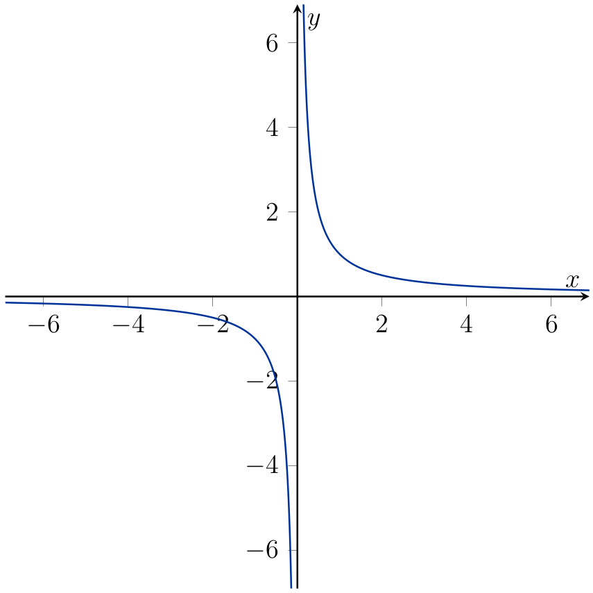
_images/1%2Cx.png — Fig. 2.3 Graph of $f(x) = \frac{1}{x}$.#

Prove rigorously that $\lim_{x \rightarrow 0^-}f(x) = - \infty$, and $\lim_{x \rightarrow 0^+}f(x) = \infty$.